Custom emitters distribution#
import numpy as np
import jetset
print('tested on jetset',jetset.__version__)
tested on jetset 1.3.0rc7
The user can build custom emitters distributions using the EmittersDistribution class. The following examples show how to implement it
Building the custom distribution#
from jetset.jet_emitters import EmittersDistribution
you need to define a function that describes your functional form (use numpy functions to make the code more performant)
def distr_func_super_exp(gamma,gamma_cut,s,a):
    return np.power(gamma,-s)*np.exp(-(1/a)*(gamma/gamma_cut)**a)
then you have to link the parmeters in your funtcion to a paramters of
the EmittersDistribution class.
Note
It is important to note that each parameter has the proper par_type string, and it is important to properly set this par_type if you want to have good results using the phenomenological constraining process.
Have a look at the predefined model to understand how to set the par_type` string. As a general rule:
the slope of the power law that starts from
gminshould be definedLE_spectral_slopeany slope of the power law above the break should be defined as
HE_spectral_slopevalues of gamma defining the transition from a power law trend toward a curved trend (including cut-off) should be defined as
turn-over-energycurvature in log-parabolic trends and/or super-exp exponent, should be defined as ‘spectral_curvature’
the spectral_type=``user_defined`` will not work for phenomenological constraining:
print('allowed_sepctral types for phenomenological constraining',EmittersDistribution.spectral_types_obs_constrain())
allowed_sepctral types for phenomenological constraining ['bkn', 'plc', 'lp', 'lppl', 'pl', 'lpep', 'array']
n_e_super_exp=EmittersDistribution('super_exp',spectral_type='user_defined')
n_e_super_exp.add_par('gamma_cut',par_type='turn-over-energy',val=50000.,vmin=1., vmax=None, unit='lorentz-factor')
n_e_super_exp.add_par('s',par_type='LE_spectral_slope',val=2.3,vmin=-10., vmax=10, unit='')
n_e_super_exp.add_par('a',par_type='spectral_curvature',val=1.8,vmin=0., vmax=100., unit='')
now you have to link your defined functional form to the
EmittersDistribution class.
n_e_super_exp.set_distr_func(distr_func_super_exp)
parameters can be easily set
n_e_super_exp.parameters.s.val=.4
n_e_super_exp.parameters.s.val=2.0
n_e_super_exp.parameters.gamma_cut.val=1E5
n_e_super_exp.normalize=True
n_e_super_exp.parameters.gmax.val=1E6
n_e_super_exp.parameters.show_pars()
| name | par type | units | val | phys. bound. min | phys. bound. max | log | frozen |
|---|---|---|---|---|---|---|---|
| gmin | low-energy-cut-off | lorentz-factor* | 2.000000e+00 | 1.000000e+00 | 1.000000e+09 | False | False |
| gmax | high-energy-cut-off | lorentz-factor* | 1.000000e+06 | 1.000000e+00 | 1.000000e+15 | False | False |
| N | emitters_density | 1 / cm3 | 1.000000e+02 | 0.000000e+00 | -- | False | False |
| gamma_cut | turn-over-energy | lorentz-factor* | 1.000000e+05 | 1.000000e+00 | -- | False | False |
| s | LE_spectral_slope | 2.000000e+00 | -1.000000e+01 | 1.000000e+01 | False | False | |
| a | spectral_curvature | 1.800000e+00 | 0.000000e+00 | 1.000000e+02 | False | False |
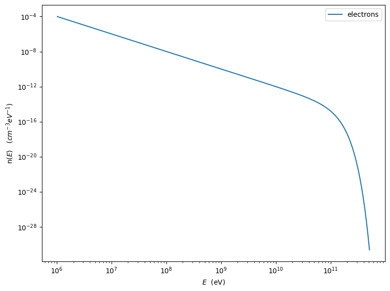
p=n_e_super_exp.plot()
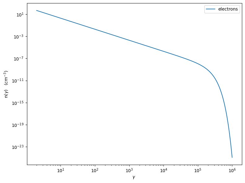
p=n_e_super_exp.plot(energy_unit='eV')
here we define a bkn power-law
def distr_func_bkn(gamma_break,gamma,s1,s2):
return np.power(gamma,-s1)*(1.+(gamma/gamma_break))**(-(s2-s1))
n_e_bkn=EmittersDistribution('bkn',spectral_type='bkn')
n_e_bkn.add_par('gamma_break',par_type='turn-over-energy',val=1E3,vmin=1., vmax=None, unit='lorentz-factor')
n_e_bkn.add_par('s1',par_type='LE_spectral_slope',val=2.5,vmin=-10., vmax=10, unit='')
n_e_bkn.add_par('s2',par_type='HE_spectral_slope',val=3.2,vmin=-10., vmax=10, unit='')
n_e_bkn.set_distr_func(distr_func_bkn)
n_e_bkn.parameters.show_pars()
n_e_bkn.parameters.s1.val=2.0
n_e_bkn.parameters.s2.val=3.5
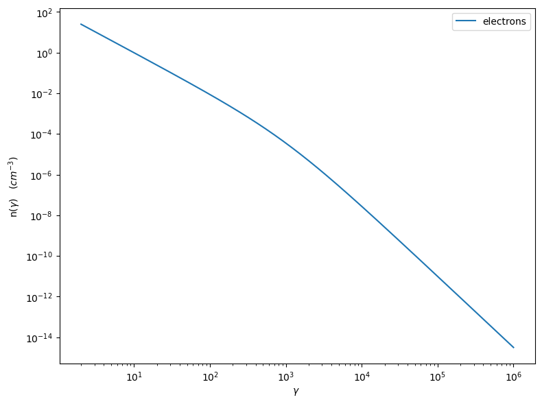
p=n_e_bkn.plot()
| name | par type | units | val | phys. bound. min | phys. bound. max | log | frozen |
|---|---|---|---|---|---|---|---|
| gmin | low-energy-cut-off | lorentz-factor* | 2.000000e+00 | 1.000000e+00 | 1.000000e+09 | False | False |
| gmax | high-energy-cut-off | lorentz-factor* | 1.000000e+06 | 1.000000e+00 | 1.000000e+15 | False | False |
| N | emitters_density | 1 / cm3 | 1.000000e+02 | 0.000000e+00 | -- | False | False |
| gamma_break | turn-over-energy | lorentz-factor* | 1.000000e+03 | 1.000000e+00 | -- | False | False |
| s1 | LE_spectral_slope | 2.500000e+00 | -1.000000e+01 | 1.000000e+01 | False | False | |
| s2 | HE_spectral_slope | 3.200000e+00 | -1.000000e+01 | 1.000000e+01 | False | False |
Passing the custom distribution to the Jet class#
The user created distribution can be passed the Jet object, when the object is instantiated, or after
Passing the custom distribution to the Jet class at instantiation time#
from jetset.jet_model import Jet
my_jet=Jet(electron_distribution=n_e_bkn)
===> setting C threads to 12
Note
now the n_e_bkn will be deep copied, so changes applied to the one passed to the model will not affect the original one
my_jet.parameters.N.val=5E4
my_jet.show_model()
my_jet.IC_nu_size=100
my_jet.eval()
--------------------------------------------------------------------------------
model description:
--------------------------------------------------------------------------------
type: Jet
name: jet_leptonic
geometry: spherical

electrons distribution:
 type: bkn
 gamma energy grid size:  201
 gmin grid : 2.000000e+00
 gmax grid : 1.000000e+06
 normalization:  False
 log-values:  False
 ratio of cold protons to relativistic electrons: 1.000000e+00

radiative fields:
 seed photons grid size:  100
 IC emission grid size:  100
 source emissivity lower bound :  1.000000e-120
 spectral components:
   name:Sum, state: on
   name:Sum, hidden: False
   name:Sync, state: self-abs
   name:Sync, hidden: False
   name:SSC, state: on
   name:SSC, hidden: False
external fields transformation method: blob

SED info:
 nu grid size jetkernel: 1000
 nu size: 500
 nu mix (Hz): 1.000000e+06
 nu max (Hz): 1.000000e+30

flux plot lower bound   :  1.000000e-30

--------------------------------------------------------------------------------
| model name | name | par type | units | val | phys. bound. min | phys. bound. max | log | frozen |
|---|---|---|---|---|---|---|---|---|
| jet_leptonic | R | region_size | cm | 5.000000e+15 | 1.000000e+03 | 1.000000e+30 | False | False |
| jet_leptonic | R_H | region_position | cm | 1.000000e+17 | 0.000000e+00 | -- | False | True |
| jet_leptonic | B | magnetic_field | gauss | 1.000000e-01 | 0.000000e+00 | -- | False | False |
| jet_leptonic | NH_cold_to_rel_e | cold_p_to_rel_e_ratio | 1.000000e+00 | 0.000000e+00 | -- | False | True | |
| jet_leptonic | beam_obj | beaming | 1.000000e+01 | 1.000000e-04 | -- | False | False | |
| jet_leptonic | z_cosm | redshift | 1.000000e-01 | 0.000000e+00 | -- | False | False | |
| jet_leptonic | gmin | low-energy-cut-off | lorentz-factor* | 2.000000e+00 | 1.000000e+00 | 1.000000e+09 | False | False |
| jet_leptonic | gmax | high-energy-cut-off | lorentz-factor* | 1.000000e+06 | 1.000000e+00 | 1.000000e+15 | False | False |
| jet_leptonic | N | emitters_density | 1 / cm3 | 5.000000e+04 | 0.000000e+00 | -- | False | False |
| jet_leptonic | gamma_break | turn-over-energy | lorentz-factor* | 1.000000e+03 | 1.000000e+00 | -- | False | False |
| jet_leptonic | s1 | LE_spectral_slope | 2.000000e+00 | -1.000000e+01 | 1.000000e+01 | False | False | |
| jet_leptonic | s2 | HE_spectral_slope | 3.500000e+00 | -1.000000e+01 | 1.000000e+01 | False | False |
--------------------------------------------------------------------------------
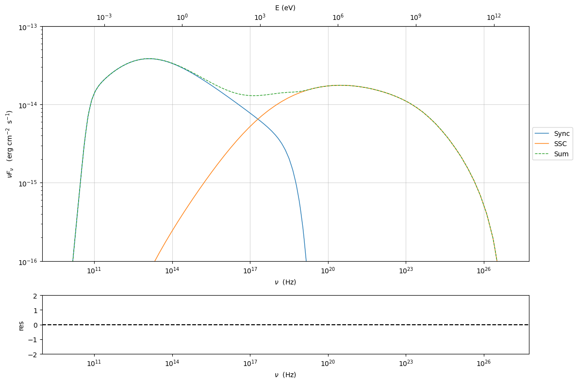
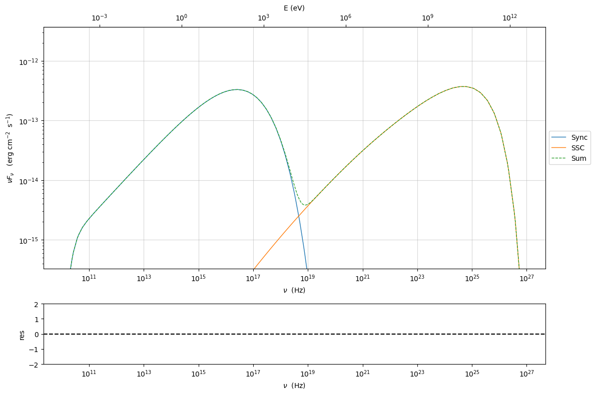
Since as default, the Nomralization is false, let’s check the actual
number density of particles and conpare it to the parameter N
print('N_particle=',my_jet.emitters_distribution.eval_N(),'N parameter=',my_jet.parameters.N.val)
N_particle= 24608.46344775512 N parameter= 50000.0
Note
N_particle is different from N, because the distribution is not normalized
my_jet.eval()
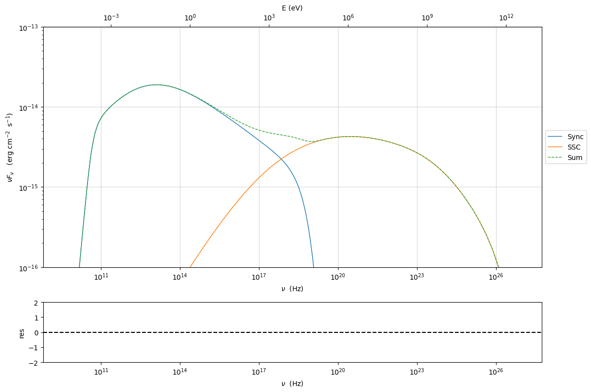
p=my_jet.plot_model()
p.setlim(y_min=1E-16,y_max=1E-13)
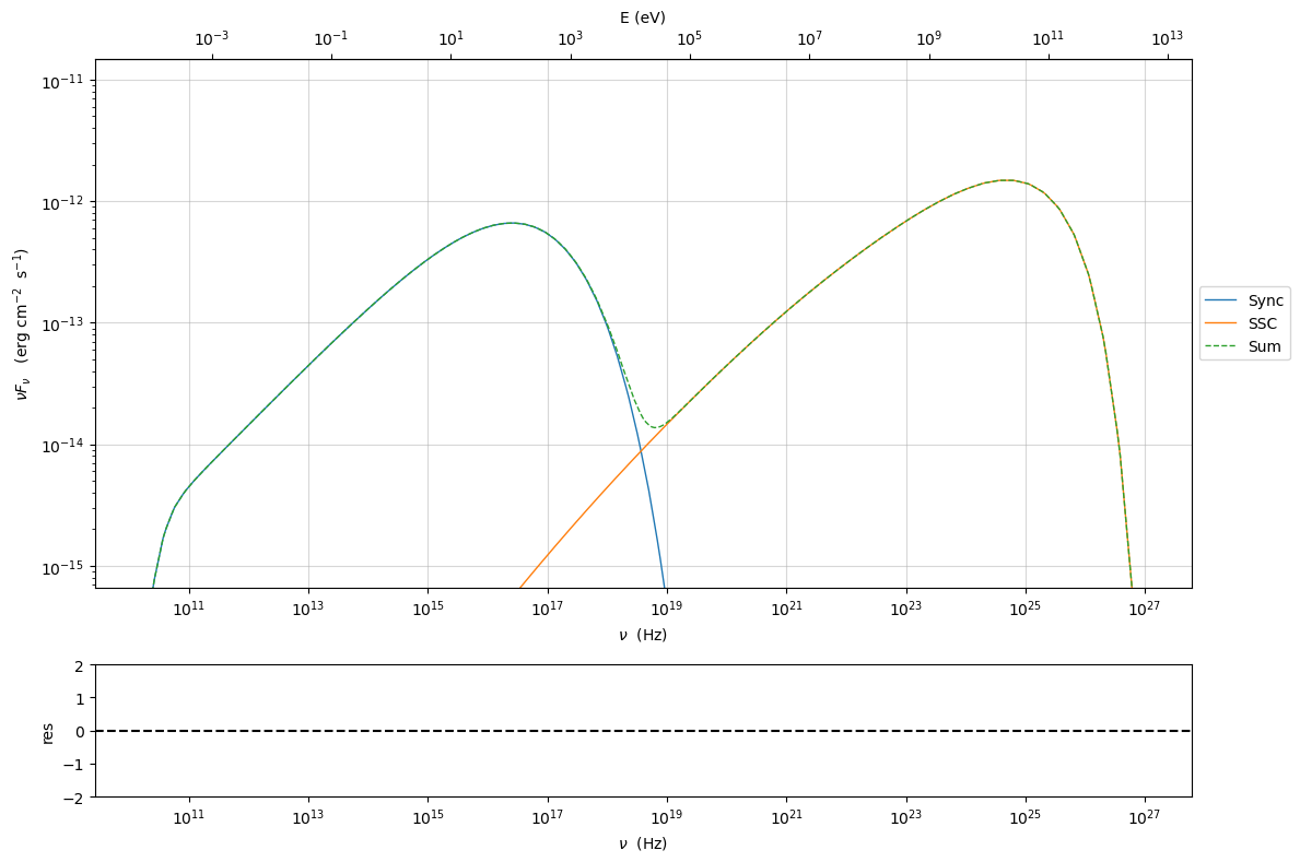
Now we switch on the normalization for the emetters distribtuion, and we keep all the parameters unchanged, including N
my_jet.Norm_distr = True
my_jet.parameters.N.val=5E4
my_jet.show_model()
my_jet.IC_nu_size=100
my_jet.eval()
--------------------------------------------------------------------------------
model description:
--------------------------------------------------------------------------------
type: Jet
name: jet_leptonic
geometry: spherical

electrons distribution:
 type: bkn
 gamma energy grid size:  201
 gmin grid : 2.000000e+00
 gmax grid : 1.000000e+06
 normalization:  True
 log-values:  False
 ratio of cold protons to relativistic electrons: 1.000000e+00

radiative fields:
 seed photons grid size:  100
 IC emission grid size:  100
 source emissivity lower bound :  1.000000e-120
 spectral components:
   name:Sum, state: on
   name:Sum, hidden: False
   name:Sync, state: self-abs
   name:Sync, hidden: False
   name:SSC, state: on
   name:SSC, hidden: False
external fields transformation method: blob

SED info:
 nu grid size jetkernel: 1000
 nu size: 500
 nu mix (Hz): 1.000000e+06
 nu max (Hz): 1.000000e+30

flux plot lower bound   :  1.000000e-30

--------------------------------------------------------------------------------
| model name | name | par type | units | val | phys. bound. min | phys. bound. max | log | frozen |
|---|---|---|---|---|---|---|---|---|
| jet_leptonic | R | region_size | cm | 5.000000e+15 | 1.000000e+03 | 1.000000e+30 | False | False |
| jet_leptonic | R_H | region_position | cm | 1.000000e+17 | 0.000000e+00 | -- | False | True |
| jet_leptonic | B | magnetic_field | gauss | 1.000000e-01 | 0.000000e+00 | -- | False | False |
| jet_leptonic | NH_cold_to_rel_e | cold_p_to_rel_e_ratio | 1.000000e+00 | 0.000000e+00 | -- | False | True | |
| jet_leptonic | beam_obj | beaming | 1.000000e+01 | 1.000000e-04 | -- | False | False | |
| jet_leptonic | z_cosm | redshift | 1.000000e-01 | 0.000000e+00 | -- | False | False | |
| jet_leptonic | gmin | low-energy-cut-off | lorentz-factor* | 2.000000e+00 | 1.000000e+00 | 1.000000e+09 | False | False |
| jet_leptonic | gmax | high-energy-cut-off | lorentz-factor* | 1.000000e+06 | 1.000000e+00 | 1.000000e+15 | False | False |
| jet_leptonic | N | emitters_density | 1 / cm3 | 5.000000e+04 | 0.000000e+00 | -- | False | False |
| jet_leptonic | gamma_break | turn-over-energy | lorentz-factor* | 1.000000e+03 | 1.000000e+00 | -- | False | False |
| jet_leptonic | s1 | LE_spectral_slope | 2.000000e+00 | -1.000000e+01 | 1.000000e+01 | False | False | |
| jet_leptonic | s2 | HE_spectral_slope | 3.500000e+00 | -1.000000e+01 | 1.000000e+01 | False | False |
--------------------------------------------------------------------------------
and we check again the actual number density of particles and conpare it to the parameter N
print('N_particle=',my_jet.emitters_distribution.eval_N(),'N parameter=',my_jet.parameters.N.val)
N_particle= 50000.0 N parameter= 50000.0
Note
N_particle and N now are the same, because the distribution is normalized
p=my_jet.plot_model()
p.setlim(y_min=1E-16,y_max=1E-13)
Passing the custom distribution to an already existing Jet object#
from jetset.jet_model import Jet
import copy
my_jet=Jet(electron_distribution='lppl')
===> setting C threads to 12
my_jet.emitters_distribution.parameters
| name | par type | units | val | phys. bound. min | phys. bound. max | log | frozen |
|---|---|---|---|---|---|---|---|
| gmin | low-energy-cut-off | lorentz-factor* | 2.000000e+00 | 1.000000e+00 | 1.000000e+09 | False | False |
| gmax | high-energy-cut-off | lorentz-factor* | 1.000000e+06 | 1.000000e+00 | 1.000000e+15 | False | False |
| N | emitters_density | 1 / cm3 | 1.000000e+02 | 0.000000e+00 | -- | False | False |
| gamma0_log_parab | turn-over-energy | lorentz-factor* | 1.000000e+04 | 1.000000e+00 | 1.000000e+09 | False | False |
| s | LE_spectral_slope | 2.000000e+00 | -1.000000e+01 | 1.000000e+01 | False | False | |
| r | spectral_curvature | 4.000000e-01 | -1.500000e+01 | 1.500000e+01 | False | False |
None
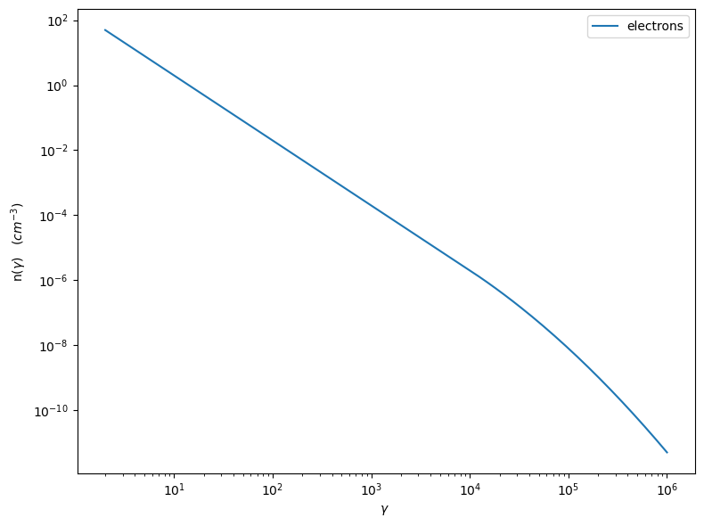
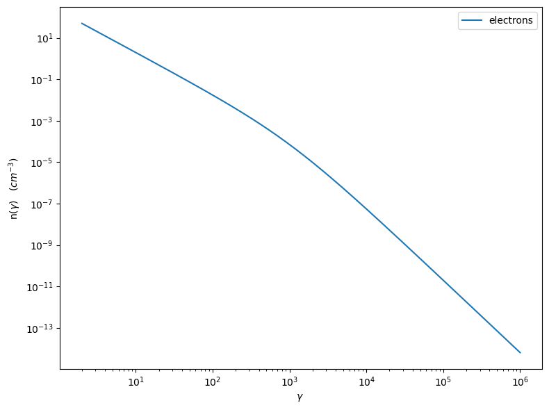
my_jet.emitters_distribution.plot()
<jetset.plot_sedfit.PlotPdistr at 0x14eb17190>
Now we update the emitters_distribution member with our custom
distribution
my_jet.emitters_distribution=n_e_bkn
my_jet.Norm_distr = True
my_jet.emitters_distribution.parameters
| name | par type | units | val | phys. bound. min | phys. bound. max | log | frozen |
|---|---|---|---|---|---|---|---|
| gmin | low-energy-cut-off | lorentz-factor* | 2.000000e+00 | 1.000000e+00 | 1.000000e+09 | False | False |
| gmax | high-energy-cut-off | lorentz-factor* | 1.000000e+06 | 1.000000e+00 | 1.000000e+15 | False | False |
| N | emitters_density | 1 / cm3 | 1.000000e+02 | 0.000000e+00 | -- | False | False |
| gamma_break | turn-over-energy | lorentz-factor* | 1.000000e+03 | 1.000000e+00 | -- | False | False |
| s1 | LE_spectral_slope | 2.000000e+00 | -1.000000e+01 | 1.000000e+01 | False | False | |
| s2 | HE_spectral_slope | 3.500000e+00 | -1.000000e+01 | 1.000000e+01 | False | False |
None
my_jet.emitters_distribution.plot()
<jetset.plot_sedfit.PlotPdistr at 0x14e334ee0>
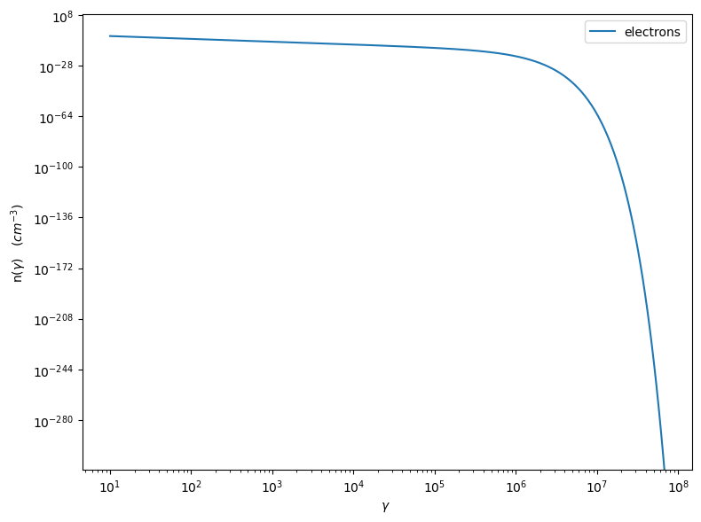
Building a distribution from an external array#
Here we just build two arrays, but you can pass any n_gamma and
gamma array wit the same size, and with gamma>1 and
n_gamma>0
from jetset.jet_emitters import EmittersArrayDistribution
import numpy as np

# gamma array
gamma = np.logspace(1, 8, 500)

# gamma array this is n(\gamma) in 1/cm^3/gamma
n_gamma = gamma ** -2 * 1E-5 * np.exp(-gamma / 1E5)

N1 = np.trapz(n_gamma, gamma)

n_distr = EmittersArrayDistribution(name='array_distr', emitters_type='electrons', gamma_array=gamma, n_gamma_array=n_gamma,normalize=False)

N2 = np.trapz(n_distr._array_n_gamma, n_distr._array_gamma)
N1 and N2 are used only for the purpose of checking, you can
skip them
p=n_distr.plot()
my_jet = Jet(emitters_distribution=n_distr, verbose=False)
my_jet.show_model()
===> setting C threads to 12

--------------------------------------------------------------------------------
model description:
--------------------------------------------------------------------------------
type: Jet
name: jet_leptonic
geometry: spherical

electrons distribution:
 type: array_distr
 gamma energy grid size:  501
 gmin grid : 1.000000e+01
 gmax grid : 1.000000e+08
 normalization:  False
 log-values:  False
 ratio of cold protons to relativistic electrons: 1.000000e+00

radiative fields:
 seed photons grid size:  100
 IC emission grid size:  100
 source emissivity lower bound :  1.000000e-120
 spectral components:
   name:Sum, state: on
   name:Sum, hidden: False
   name:Sync, state: self-abs
   name:Sync, hidden: False
   name:SSC, state: on
   name:SSC, hidden: False
external fields transformation method: blob

SED info:
 nu grid size jetkernel: 1000
 nu size: 500
 nu mix (Hz): 1.000000e+06
 nu max (Hz): 1.000000e+30

flux plot lower bound   :  1.000000e-30

--------------------------------------------------------------------------------
| model name | name | par type | units | val | phys. bound. min | phys. bound. max | log | frozen |
|---|---|---|---|---|---|---|---|---|
| jet_leptonic | R | region_size | cm | 5.000000e+15 | 1.000000e+03 | 1.000000e+30 | False | False |
| jet_leptonic | R_H | region_position | cm | 1.000000e+17 | 0.000000e+00 | -- | False | True |
| jet_leptonic | B | magnetic_field | gauss | 1.000000e-01 | 0.000000e+00 | -- | False | False |
| jet_leptonic | NH_cold_to_rel_e | cold_p_to_rel_e_ratio | 1.000000e+00 | 0.000000e+00 | -- | False | True | |
| jet_leptonic | beam_obj | beaming | 1.000000e+01 | 1.000000e-04 | -- | False | False | |
| jet_leptonic | z_cosm | redshift | 1.000000e-01 | 0.000000e+00 | -- | False | False | |
| jet_leptonic | gmin | low-energy-cut-off | lorentz-factor* | 1.000000e+01 | 1.000000e+00 | 1.000000e+09 | False | False |
| jet_leptonic | gmax | high-energy-cut-off | lorentz-factor* | 1.000000e+08 | 1.000000e+00 | 1.000000e+15 | False | False |
| jet_leptonic | N | scaling_factor | 1.000000e+00 | 0.000000e+00 | -- | False | False |
--------------------------------------------------------------------------------
you can also skip the next cell, it is just to check
N3 = np.trapz(my_jet.emitters_distribution.n_gamma_e, my_jet.emitters_distribution.gamma_e)

np.testing.assert_allclose(N1, N2, rtol=1E-5)
np.testing.assert_allclose(N1, N3, rtol=1E-2)
np.testing.assert_allclose(N1, my_jet.emitters_distribution.eval_N(), rtol=1E-2)
N will act as a scaling factor for the array when normalization is
set to False
my_jet.parameters.N.val=1E9
print('this is the actual number of emitters dendisty %2.2f'%my_jet.emitters_distribution.eval_N(),'this the scaling factor',my_jet.parameters.N.val)
this is the actual number of emitters dendisty 999.56 this the scaling factor 1000000000.0
my_jet.eval()
p=my_jet.plot_model()
you can still normalize the distribution
my_jet.Norm_distr = True
my_jet.parameters.N.val=2000
print('this is the actaul number of emitters dendisty %2.2f'%my_jet.emitters_distribution.eval_N(),'this the scaling factor',my_jet.parameters.N.val)
this is the actaul number of emitters dendisty 2000.00 this the scaling factor 2000
my_jet.eval()
p=my_jet.plot_model()
my_jet.save_model('test_jet_custom_emitters_array.pkl')
new_jet = Jet.load_model('test_jet_custom_emitters_array.pkl')
===> setting C threads to 12
new_jet.eval()
p=new_jet.plot_model()
