Physical setup#

import jetset
print('tested on jetset',jetset.__version__)

tested on jetset 1.3.0rc7

In this section we describe how to build a model of jet able to reproduce SSC/EC emission processes, using the Jet class from the jet_model module. This class, through a flexible and intuitive interface, allows access to the C numerical code which provides an accurate and fast computation of the synchrotron and inverse Compton processes.

Basic setup and C threads#

A jet instance can be built using the the Jet class, instantiating the object in the following way:

from jetset.jet_model import Jet
my_jet=Jet(name='test',electron_distribution='lppl')

===> setting C threads to 12

This instruction will create:

a Jet object with name test,
using as electron distribution the lppl model, that is a log-parabola with a low-energy power-law branch.

(a working directory jet_wd will be created, this directory can be deleted when all the processes of your script are done, and will be removed in next versions)

C threads#

Important

Starting from version 1.3.0 the Jet class, and all the derived classes, perform the C computation using threads. This increases. the computational speed Each time you create a new Jet object, you will get a log message reporting how many C threads have been created. The number of threads is automatically determined according to the number of cores and threads of your computation. You can revert back to a single thread using the set_num_c_threads and passing the number of threads by your CPU. Increasing the number of threads above the number of threads supported by your CPU will not improve the performance.

Switch back to a single C thread

my_jet.set_num_c_threads(1)

===> setting C threads to 1

Set a custom number of C treads

my_jet.set_num_c_threads(8)

===> setting C threads to 8

let’s try how changes the computational speed with the number of threads

my_jet.set_num_c_threads(1)

===> setting C threads to 1

%timeit my_jet.eval()

71.8 ms ± 430 µs per loop (mean ± std. dev. of 7 runs, 10 loops each)

my_jet.set_num_c_threads(8)

===> setting C threads to 8

%timeit my_jet.eval()

26.7 ms ± 139 µs per loop (mean ± std. dev. of 7 runs, 10 loops each)

my_jet.set_num_c_threads(10)

===> setting C threads to 10

%timeit my_jet.eval()

29.9 ms ± 11.3 ms per loop (mean ± std. dev. of 7 runs, 10 loops each)

my_jet.set_num_c_threads(20)

===> setting C threads to 20

%timeit my_jet.eval()

24.9 ms ± 456 µs per loop (mean ± std. dev. of 7 runs, 10 loops each)

as you can see, the computational speed saturates at 8 threads, to a value fo ~ 20 ms per computation ~50 computation per second, on an 2/6 GHz 6-Core Intel Core i7 (I7-9750H)

basic configurations#

For a list of possible electron distributions you can run the command

Jet.available_electron_distributions()

lp: log-parabola
pl: powerlaw
lppl: log-parabola with low-energy powerlaw branch
lpep: log-parabola defined by peak energy
plc: powerlaw with cut-off
bkn: broken powerlaw
superexp: powerlaw with super-exp cut-off

to view all the paramters of the jet model:

my_jet.show_pars()

Table length=12

model name	name	par type	units	val	phys. bound. min	phys. bound. max	log	frozen
test	R	region_size	cm	5.000000e+15	1.000000e+03	1.000000e+30	False	False
test	R_H	region_position	cm	1.000000e+17	0.000000e+00	--	False	True
test	B	magnetic_field	gauss	1.000000e-01	0.000000e+00	--	False	False
test	NH_cold_to_rel_e	cold_p_to_rel_e_ratio		1.000000e+00	0.000000e+00	--	False	True
test	beam_obj	beaming		1.000000e+01	1.000000e-04	--	False	False
test	z_cosm	redshift		1.000000e-01	0.000000e+00	--	False	False
test	gmin	low-energy-cut-off	lorentz-factor*	2.000000e+00	1.000000e+00	1.000000e+09	False	False
test	gmax	high-energy-cut-off	lorentz-factor*	1.000000e+06	1.000000e+00	1.000000e+15	False	False
test	N	emitters_density	1 / cm3	1.000000e+02	0.000000e+00	--	False	False
test	gamma0_log_parab	turn-over-energy	lorentz-factor*	1.000000e+04	1.000000e+00	1.000000e+09	False	False
test	s	LE_spectral_slope		2.000000e+00	-1.000000e+01	1.000000e+01	False	False
test	r	spectral_curvature		4.000000e-01	-1.500000e+01	1.500000e+01	False	False

custom electron distributions can be created by the user as described in this section of the tutorial Custom emitters distribution

Each parameter has a default value. All the parameters listed are handled by ModelParameterArray, and each parameter is an instance of the the JetParameter. class. These parameters can be visualized by the command

my_jet.parameters

Table length=12

model name	name	par type	units	val	phys. bound. min	phys. bound. max	log	frozen
test	R	region_size	cm	5.000000e+15	1.000000e+03	1.000000e+30	False	False
test	R_H	region_position	cm	1.000000e+17	0.000000e+00	--	False	True
test	B	magnetic_field	gauss	1.000000e-01	0.000000e+00	--	False	False
test	NH_cold_to_rel_e	cold_p_to_rel_e_ratio		1.000000e+00	0.000000e+00	--	False	True
test	beam_obj	beaming		1.000000e+01	1.000000e-04	--	False	False
test	z_cosm	redshift		1.000000e-01	0.000000e+00	--	False	False
test	gmin	low-energy-cut-off	lorentz-factor*	2.000000e+00	1.000000e+00	1.000000e+09	False	False
test	gmax	high-energy-cut-off	lorentz-factor*	1.000000e+06	1.000000e+00	1.000000e+15	False	False
test	N	emitters_density	1 / cm3	1.000000e+02	0.000000e+00	--	False	False
test	gamma0_log_parab	turn-over-energy	lorentz-factor*	1.000000e+04	1.000000e+00	1.000000e+09	False	False
test	s	LE_spectral_slope		2.000000e+00	-1.000000e+01	1.000000e+01	False	False
test	r	spectral_curvature		4.000000e-01	-1.500000e+01	1.500000e+01	False	False

None

and the corresponding astropy table with units can be accessed by: my_jet.parameters.par_table

This means that you can easily convert the values in the table using the units module of astropy.

Warning

Please note, that the table is built on the fly from the ModelParameterArray and each modification you do to this table will not be reflected on the actual parameters values

To get a full description of the model you can use the instruction

my_jet.show_model()

--------------------------------------------------------------------------------
model description:
--------------------------------------------------------------------------------
type: Jet
name: test
geometry: spherical

electrons distribution:
 type: lppl
 gamma energy grid size:  201
 gmin grid : 2.000000e+00
 gmax grid : 1.000000e+06
 normalization:  True
 log-values:  False
 ratio of cold protons to relativistic electrons: 1.000000e+00

radiative fields:
 seed photons grid size:  100
 IC emission grid size:  100
 source emissivity lower bound :  1.000000e-120
 spectral components:
   name:Sum, state: on
   name:Sum, hidden: False
   name:Sync, state: self-abs
   name:Sync, hidden: False
   name:SSC, state: on
   name:SSC, hidden: False
external fields transformation method: blob

SED info:
 nu grid size jetkernel: 1000
 nu size: 500
 nu mix (Hz): 1.000000e+06
 nu max (Hz): 1.000000e+30

flux plot lower bound   :  1.000000e-30

--------------------------------------------------------------------------------

Table length=12

model name	name	par type	units	val	phys. bound. min	phys. bound. max	log	frozen
test	R	region_size	cm	5.000000e+15	1.000000e+03	1.000000e+30	False	False
test	R_H	region_position	cm	1.000000e+17	0.000000e+00	--	False	True
test	B	magnetic_field	gauss	1.000000e-01	0.000000e+00	--	False	False
test	NH_cold_to_rel_e	cold_p_to_rel_e_ratio		1.000000e+00	0.000000e+00	--	False	True
test	beam_obj	beaming		1.000000e+01	1.000000e-04	--	False	False
test	z_cosm	redshift		1.000000e-01	0.000000e+00	--	False	False
test	gmin	low-energy-cut-off	lorentz-factor*	2.000000e+00	1.000000e+00	1.000000e+09	False	False
test	gmax	high-energy-cut-off	lorentz-factor*	1.000000e+06	1.000000e+00	1.000000e+15	False	False
test	N	emitters_density	1 / cm3	1.000000e+02	0.000000e+00	--	False	False
test	gamma0_log_parab	turn-over-energy	lorentz-factor*	1.000000e+04	1.000000e+00	1.000000e+09	False	False
test	s	LE_spectral_slope		2.000000e+00	-1.000000e+01	1.000000e+01	False	False
test	r	spectral_curvature		4.000000e-01	-1.500000e+01	1.500000e+01	False	False

--------------------------------------------------------------------------------

Warning

Starting from version 1.1.0, the R parameter as default is linear and not logarithmic, please update your old scripts setting R with linear values.

as you can notice, you can now access further information regarding the model, such as numerical configuration of the grid. These numerical parameters will be discussed in the :ref:`jet_numerical_guide’ section

If you want to use a cosmology model different from the default one please read the Choosing a cosmology model section. To get information regarding the current cosmological model:

my_jet.cosmo

FlatLambdaCDM(name="Planck13", H0=67.77 km / (Mpc s), Om0=0.30712, Tcmb0=2.7255 K, Neff=3.046, m_nu=[0.   0.   0.06] eV, Ob0=0.048252)

Setting the parameters#

Assume you want to change some of the parameters in your model, you can use two methods:

using the Jet.set_par() method

my_jet.set_par('B',val=0.2)
my_jet.set_par('gamma0_log_parab',val=5E3)
my_jet.set_par('gmin',val=1E2)
my_jet.set_par('gmax',val=1E8)
my_jet.set_par('R',val=1E15)
my_jet.set_par('N',val=1E3)

accessing directly the parameter

my_jet.parameters.B.val=0.2
my_jet.parameters.r.val=0.4

Investigating the electron distribution#

for setting custom electron distributions can be created by the user as described in this section of the tutorial Custom emitters distribution

my_jet.show_electron_distribution()

--------------------------------------------------------------------------------
electrons distribution:
 type: lppl
 gamma energy grid size:  201
 gmin grid : 2.000000e+00
 gmax grid : 1.000000e+06
 normalization  True
 log-values  False

Table length=12

model name	name	par type	units	val	phys. bound. min	phys. bound. max	log	frozen
test	B	magnetic_field	gauss	2.000000e-01	0.000000e+00	--	False	False
test	N	emitters_density	1 / cm3	1.000000e+03	0.000000e+00	--	False	False
test	NH_cold_to_rel_e	cold_p_to_rel_e_ratio		1.000000e+00	0.000000e+00	--	False	True
test	R	region_size	cm	1.000000e+15	1.000000e+03	1.000000e+30	False	False
test	R_H	region_position	cm	1.000000e+17	0.000000e+00	--	False	True
test	beam_obj	beaming		1.000000e+01	1.000000e-04	--	False	False
test	gamma0_log_parab	turn-over-energy	lorentz-factor*	5.000000e+03	1.000000e+00	1.000000e+09	False	False
test	gmax	high-energy-cut-off	lorentz-factor*	1.000000e+08	1.000000e+00	1.000000e+15	False	False
test	gmin	low-energy-cut-off	lorentz-factor*	1.000000e+02	1.000000e+00	1.000000e+09	False	False
test	r	spectral_curvature		4.000000e-01	-1.500000e+01	1.500000e+01	False	False
test	s	LE_spectral_slope		2.000000e+00	-1.000000e+01	1.000000e+01	False	False
test	z_cosm	redshift		1.000000e-01	0.000000e+00	--	False	False

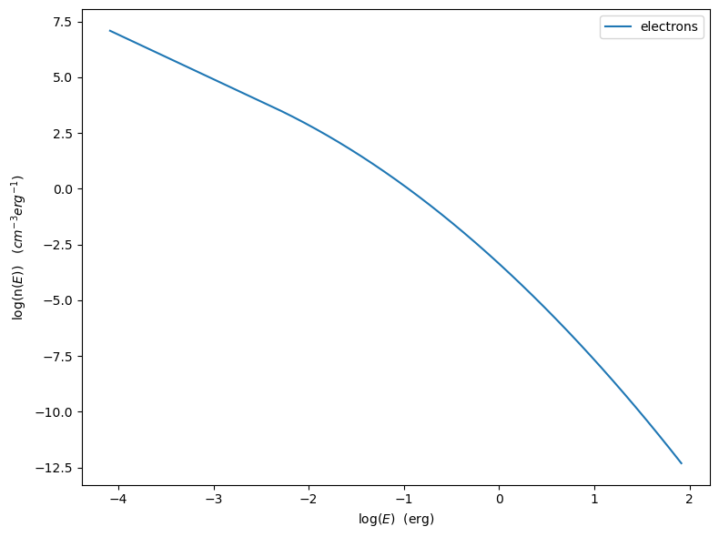
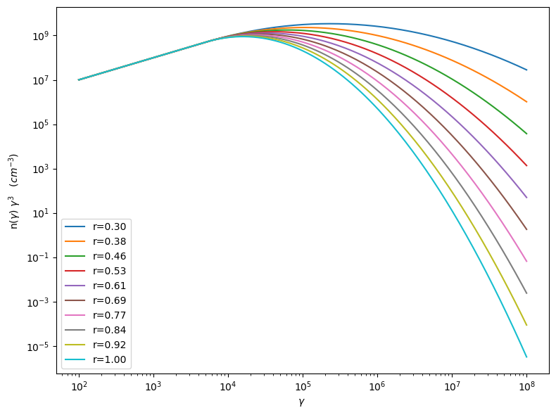
p=my_jet.electron_distribution.plot3p()

../../../../_images/Jet_example_phys_SSC_49_0.png

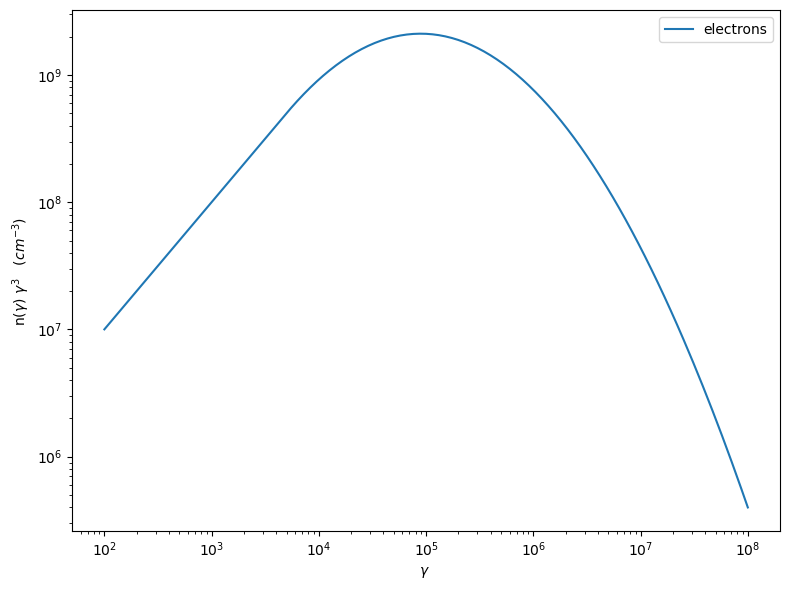
p=my_jet.electron_distribution.plot3p(energy_unit='eV')

../../../../_images/Jet_example_phys_SSC_50_0.png

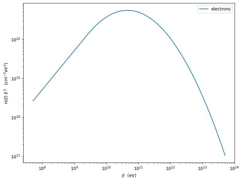
p=my_jet.electron_distribution.plot2p(energy_unit='erg')

../../../../_images/Jet_example_phys_SSC_51_0.png

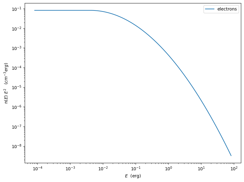
to obtain a loglog plot, pass loglog=True to the plot method

p=my_jet.electron_distribution.plot(energy_unit='erg',loglog=True)

../../../../_images/Jet_example_phys_SSC_53_0.png

import numpy as np
p=None
for r in np.linspace(0.3,1,10):
    my_jet.parameters.r.val=r
    _l='r=%2.2f'%r
    if p is None:
        p=my_jet.electron_distribution.plot3p(label=_l)
    else:
        p=my_jet.electron_distribution.plot3p(p,label=_l)

../../../../_images/Jet_example_phys_SSC_54_0.png

Using log values for electron distribution parameters#

my_jet=Jet(name='test',electron_distribution='lppl',electron_distribution_log_values=True)
my_jet.show_model()

===> setting C threads to 12

--------------------------------------------------------------------------------
model description:
--------------------------------------------------------------------------------
type: Jet
name: test
geometry: spherical

electrons distribution:
 type: lppl
 gamma energy grid size:  201
 gmin grid : 2.000000e+00
 gmax grid : 1.000000e+06
 normalization:  True
 log-values:  True
 ratio of cold protons to relativistic electrons: 1.000000e+00

radiative fields:
 seed photons grid size:  100
 IC emission grid size:  100
 source emissivity lower bound :  1.000000e-120
 spectral components:
   name:Sum, state: on
   name:Sum, hidden: False
   name:Sync, state: self-abs
   name:Sync, hidden: False
   name:SSC, state: on
   name:SSC, hidden: False
external fields transformation method: blob

SED info:
 nu grid size jetkernel: 1000
 nu size: 500
 nu mix (Hz): 1.000000e+06
 nu max (Hz): 1.000000e+30

flux plot lower bound   :  1.000000e-30

--------------------------------------------------------------------------------

Table length=12

model name	name	par type	units	val	phys. bound. min	phys. bound. max	log	frozen
test	R	region_size	cm	5.000000e+15	1.000000e+03	1.000000e+30	False	False
test	R_H	region_position	cm	1.000000e+17	0.000000e+00	--	False	True
test	B	magnetic_field	gauss	1.000000e-01	0.000000e+00	--	False	False
test	NH_cold_to_rel_e	cold_p_to_rel_e_ratio		1.000000e+00	0.000000e+00	--	False	True
test	beam_obj	beaming		1.000000e+01	1.000000e-04	--	False	False
test	z_cosm	redshift		1.000000e-01	0.000000e+00	--	False	False
test	gmin	low-energy-cut-off	lorentz-factor*	3.010300e-01	0.000000e+00	9.000000e+00	True	False
test	gmax	high-energy-cut-off	lorentz-factor*	6.000000e+00	0.000000e+00	1.500000e+01	True	False
test	N	emitters_density	1 / cm3	1.000000e+02	0.000000e+00	--	False	False
test	gamma0_log_parab	turn-over-energy	lorentz-factor*	4.000000e+00	0.000000e+00	9.000000e+00	True	False
test	s	LE_spectral_slope		2.000000e+00	-1.000000e+01	1.000000e+01	False	False
test	r	spectral_curvature		4.000000e-01	-1.500000e+01	1.500000e+01	False	False

--------------------------------------------------------------------------------

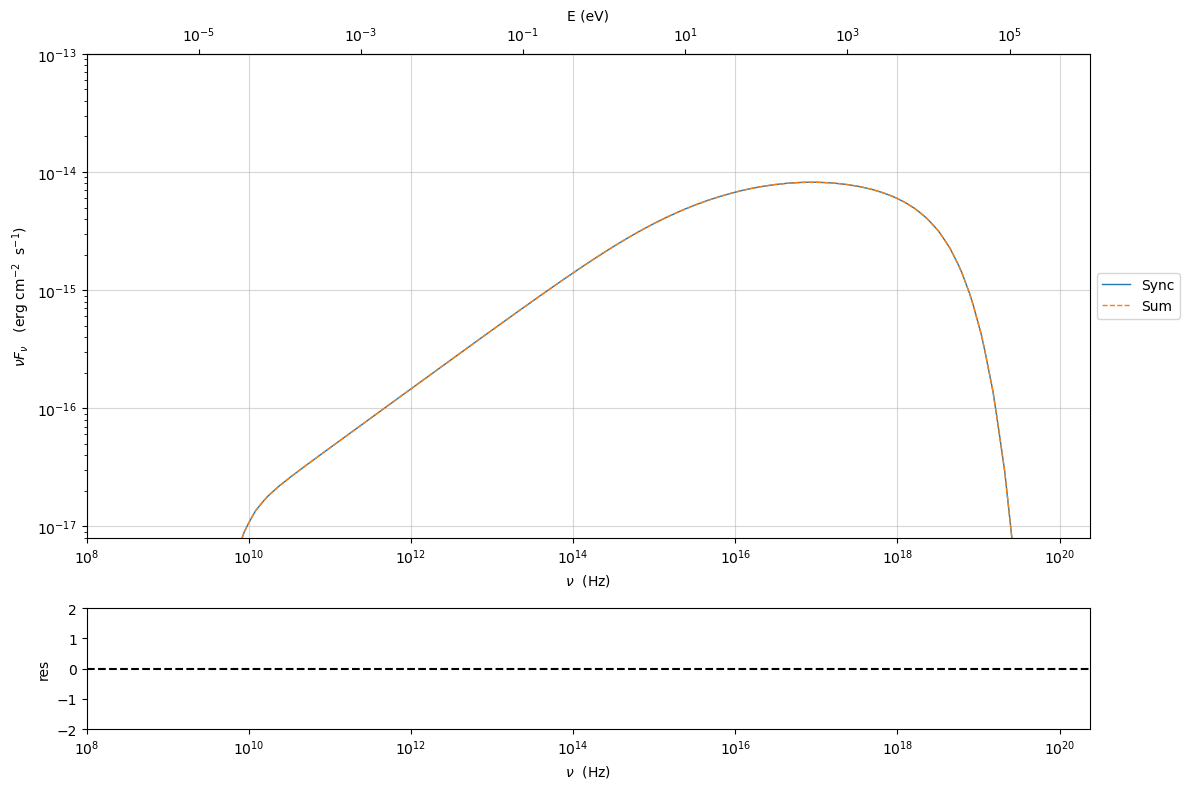
Evaluate and plot the model#

At this point we can evaluate the emission for this jet model using the instruction

my_jet.eval()

my_jet.show_pars()

Table length=12

model name	name	par type	units	val	phys. bound. min	phys. bound. max	log	frozen
test	R	region_size	cm	5.000000e+15	1.000000e+03	1.000000e+30	False	False
test	R_H	region_position	cm	1.000000e+17	0.000000e+00	--	False	True
test	B	magnetic_field	gauss	1.000000e-01	0.000000e+00	--	False	False
test	NH_cold_to_rel_e	cold_p_to_rel_e_ratio		1.000000e+00	0.000000e+00	--	False	True
test	beam_obj	beaming		1.000000e+01	1.000000e-04	--	False	False
test	z_cosm	redshift		1.000000e-01	0.000000e+00	--	False	False
test	gmin	low-energy-cut-off	lorentz-factor*	3.010300e-01	0.000000e+00	9.000000e+00	True	False
test	gmax	high-energy-cut-off	lorentz-factor*	6.000000e+00	0.000000e+00	1.500000e+01	True	False
test	N	emitters_density	1 / cm3	1.000000e+02	0.000000e+00	--	False	False
test	gamma0_log_parab	turn-over-energy	lorentz-factor*	4.000000e+00	0.000000e+00	9.000000e+00	True	False
test	s	LE_spectral_slope		2.000000e+00	-1.000000e+01	1.000000e+01	False	False
test	r	spectral_curvature		4.000000e-01	-1.500000e+01	1.500000e+01	False	False

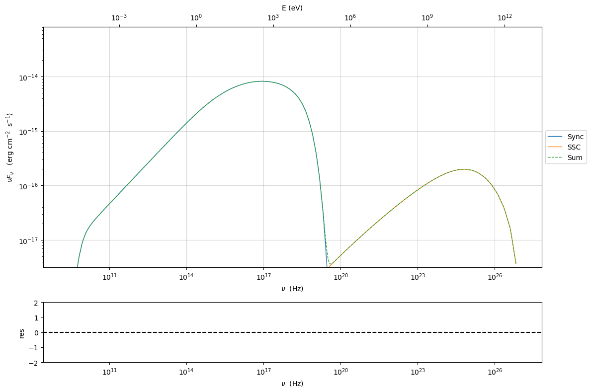
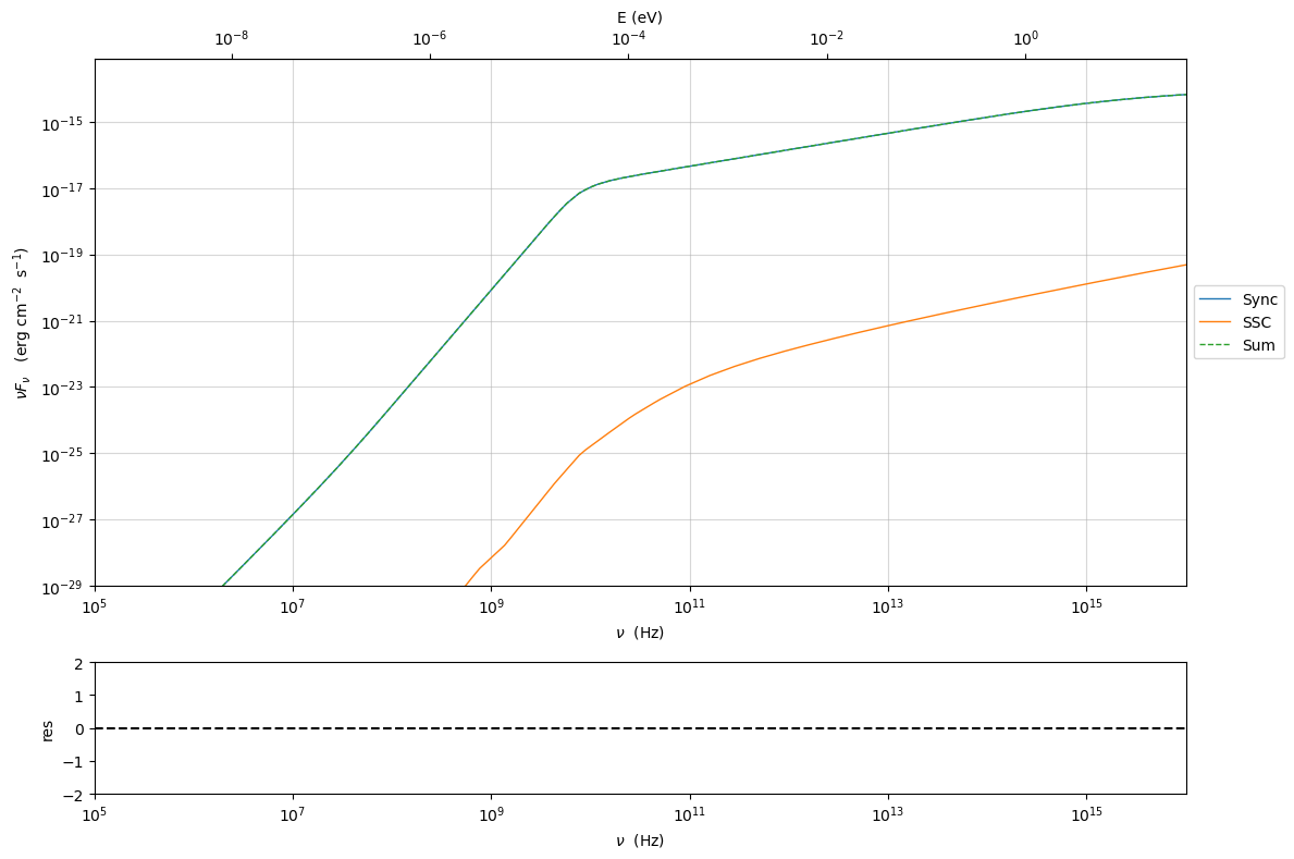
and plot the corresponding SED:

Warning

Starting from version 1.2.0 The rescale method as been replaced by the setlim methd. Please notice, that now jetset uses as defualt logarthmic axis rather than loglog plots, so, the correct way to use it is rescale(x_min=8)->setlim(x_min=1E8)

from jetset.plot_sedfit import PlotSED
my_plot=PlotSED()
my_jet.plot_model(plot_obj=my_plot)
my_plot.setlim(y_min=10**-17.5)

../../../../_images/Jet_example_phys_SSC_63_0.png

alternatively, you can call the plot_model method without passing a Plot object

my_plot=my_jet.plot_model()
my_plot.setlim(y_min=10**-17.5)

../../../../_images/Jet_example_phys_SSC_65_0.png

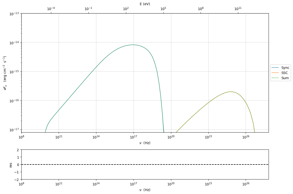
If you want to have more points on the IC spectrum you can set the numerical parameters for radiative fields(see :ref:`jet_numerical_guide’ section for more details):

my_jet.set_IC_nu_size(100)

my_jet.eval()
my_plot=my_jet.plot_model()
my_plot.setlim(y_min=10**-17.5)

../../../../_images/Jet_example_phys_SSC_68_0.png

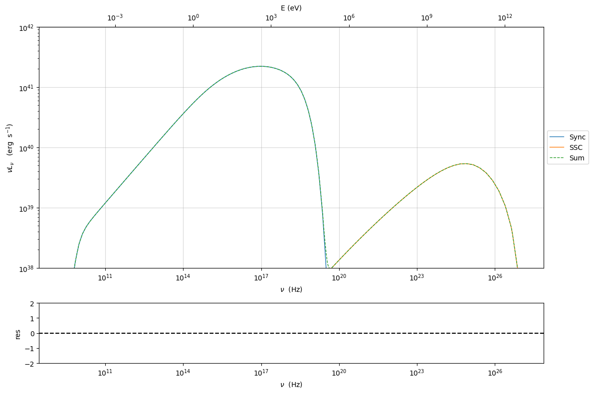
you can access the same plot, but in the rest frame of the black hole, or accretion disk, hence plotting the isotropic luminosity, by simply passing the frame kw to src

my_plot=my_jet.plot_model(frame='src')
my_plot.setlim(y_max=1E42,y_min=1E38)

../../../../_images/Jet_example_phys_SSC_70_0.png

the my_plot object returned will be built on the fly by the plot_model method

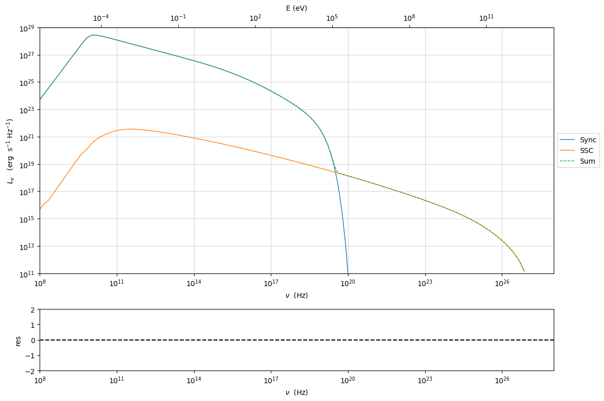
Starting from version 1.2.0 you can also plot in the Fnu or Lnu representation adding the density=True keyword to the plot_model command

my_plot=my_jet.plot_model(frame='src',density=True)
my_plot.setlim(y_max=1E29,y_min=1E11,x_min=1E8,x_max=1E28)

../../../../_images/Jet_example_phys_SSC_73_0.png

Changing the nu grid#

The SED info header displayed by the :meth:.Jet.show_model() method reports information for the SED nu_min, nu_max, nu_size and nu_grid_size.

The nu_grid_size is the internal interpolation grid used by jetkernel C code, and it should not be changed
The nu_size is the Python interpolation grid used by the Python wrapper on top of the jetkernel one, and is used only for the SEDs production and plotting.
nu_min and nu_max, are used for the boundaries of the model, and can be changed if the custom value does not cover your expected range.

Note

if the model is below the source emissivity or flux plot lower bound, then your changes on nu_min/nu_max will have no effect, and you have to decrease the source emissivity or flux plot lower bound eg:

my_jet.flux_plot_lim=1E-40
my_jet.set_emiss_lim(1E-200)

my_jet.nu_min=1E5
my_jet.nu_size=400
my_jet.nu_max=1E30

my_jet.show_model()

--------------------------------------------------------------------------------
model description:
--------------------------------------------------------------------------------
type: Jet
name: test
geometry: spherical

electrons distribution:
 type: lppl
 gamma energy grid size:  201
 gmin grid : 2.000000e+00
 gmax grid : 1.000000e+06
 normalization:  True
 log-values:  True
 ratio of cold protons to relativistic electrons: 1.000000e+00

radiative fields:
 seed photons grid size:  100
 IC emission grid size:  100
 source emissivity lower bound :  1.000000e-120
 spectral components:
   name:Sum, state: on
   name:Sum, hidden: False
   name:Sync, state: self-abs
   name:Sync, hidden: False
   name:SSC, state: on
   name:SSC, hidden: False
external fields transformation method: blob

SED info:
 nu grid size jetkernel: 1000
 nu size: 400
 nu mix (Hz): 1.000000e+05
 nu max (Hz): 1.000000e+30

flux plot lower bound   :  1.000000e-30

--------------------------------------------------------------------------------

Table length=12

model name	name	par type	units	val	phys. bound. min	phys. bound. max	log	frozen
test	R	region_size	cm	5.000000e+15	1.000000e+03	1.000000e+30	False	False
test	R_H	region_position	cm	1.000000e+17	0.000000e+00	--	False	True
test	B	magnetic_field	gauss	1.000000e-01	0.000000e+00	--	False	False
test	NH_cold_to_rel_e	cold_p_to_rel_e_ratio		1.000000e+00	0.000000e+00	--	False	True
test	beam_obj	beaming		1.000000e+01	1.000000e-04	--	False	False
test	z_cosm	redshift		1.000000e-01	0.000000e+00	--	False	False
test	gmin	low-energy-cut-off	lorentz-factor*	3.010300e-01	0.000000e+00	9.000000e+00	True	False
test	gmax	high-energy-cut-off	lorentz-factor*	6.000000e+00	0.000000e+00	1.500000e+01	True	False
test	N	emitters_density	1 / cm3	1.000000e+02	0.000000e+00	--	False	False
test	gamma0_log_parab	turn-over-energy	lorentz-factor*	4.000000e+00	0.000000e+00	9.000000e+00	True	False
test	s	LE_spectral_slope		2.000000e+00	-1.000000e+01	1.000000e+01	False	False
test	r	spectral_curvature		4.000000e-01	-1.500000e+01	1.500000e+01	False	False

--------------------------------------------------------------------------------

my_jet.eval()
import matplotlib.ticker as ticker
p=my_jet.plot_model()
p.setlim(x_min=1E5,x_max=1E16,y_min=10**-29)
plt.show()

../../../../_images/Jet_example_phys_SSC_78_0.png

if you want to to have interacitve plot:

in a jupyter notebook use:

%matplotlib notebook

in jupyter lab:

%matplotlib widget
(visit this url to setup and install: https://github.com/matplotlib/ipympl)

in an ipython terminal

from matplotlib import pylab as plt
plt.ion()

Comparing models on the same plot#

to compare the same model after changing a parameter

my_jet=Jet(name='test',electron_distribution='lppl',)
my_jet.set_par('B',val=0.2)
my_jet.set_par('gamma0_log_parab',val=5E3)
my_jet.set_par('gmin',val=1E2)
my_jet.set_par('gmax',val=1E8)
my_jet.set_par('R',val=10**14.5)
my_jet.set_par('N',val=1E3)

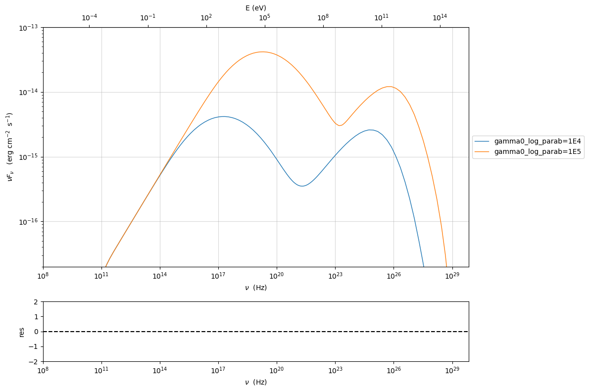
my_jet.parameters.gamma0_log_parab.val=1E4
my_jet.eval()
my_plot=my_jet.plot_model(label='gamma0_log_parab=1E4',comp='Sum')
my_jet.set_par('gamma0_log_parab',val=1.0E5)
my_jet.eval()
my_plot=my_jet.plot_model(my_plot,label='gamma0_log_parab=1E5',comp='Sum')
my_plot.setlim(y_max=1E-13,y_min=2E-17,x_min=1E8)

===> setting C threads to 12

../../../../_images/Jet_example_phys_SSC_82_1.png

Saving a plot#

to save the plot

my_plot.save('jet1.png')

Saving and loading a model#

Important

version 1.3.0 has changed the serialization of models, to be independent from changes in imported libraries, hence, models saved with previous versions might not be possible.

my_jet.save_model('test_model.pkl')

my_jet_new=Jet.load_model('test_model.pkl')

===> setting C threads to 12

Switching on/off the particle distribution normalization#

As default the electron distributions are normalized, i.e. are multiplied by a constant N_0, in such a way that :

\(\int_{\gamma_{min}}^{\gamma_{max}} n(\gamma) d\gamma =1\),

it means the the value N, refers to the actual density of emitters. If you want to chance this behavior, you can start looking at the sate of Norm_distr flag with the following command

my_jet.Norm_distr

True

and then you can switch off the normalization withe command

my_jet.switch_Norm_distr_OFF()

my_jet.Norm_distr=0

my_jet.switch_Norm_distr_ON()

my_jet.Norm_distr=1

Setting the particle density from observed Fluxes or Luminosities#

It is possible to set the density of emitting particles starting from some observed luminosity or flux (see the method Jet.set_N_from_nuFnu(), and Jet.set_N_from_nuLnu())

my_jet=Jet(name='test',electron_distribution='lppl')

===> setting C threads to 12

this is the initial value of N

my_jet.parameters.N.val

we now want to set the value of N in order that the observed synchrotron flux at a given frequency matches a target value. For example, assume that we wish to set N in order that the synchrotron flux at \(10^{15}\) Hz is exactly matching the desired value of \(10^{-14}\) ergs cm-2 s-1. We can accomplish this by using the method Jet.set_N_from_nuFnu() as follows:

my_jet.set_N_from_nuFnu(nuFnu_obs=1E-14,nu_obs=1E15)

This is the updated value of N, obtained in order to match the given flux at the given frequency

my_jet.get_par_by_name('N').val

272.4

my_jet.parameters.N.val

272.4

my_jet.parameters.show_pars()

Table length=12

model name	name	par type	units	val	phys. bound. min	phys. bound. max	log	frozen
test	R	region_size	cm	5.000000e+15	1.000000e+03	1.000000e+30	False	False
test	R_H	region_position	cm	1.000000e+17	0.000000e+00	--	False	True
test	B	magnetic_field	gauss	1.000000e-01	0.000000e+00	--	False	False
test	NH_cold_to_rel_e	cold_p_to_rel_e_ratio		1.000000e+00	0.000000e+00	--	False	True
test	beam_obj	beaming		1.000000e+01	1.000000e-04	--	False	False
test	z_cosm	redshift		1.000000e-01	0.000000e+00	--	False	False
test	gmin	low-energy-cut-off	lorentz-factor*	2.000000e+00	1.000000e+00	1.000000e+09	False	False
test	gmax	high-energy-cut-off	lorentz-factor*	1.000000e+06	1.000000e+00	1.000000e+15	False	False
test	N	emitters_density	1 / cm3	2.723756e+02	0.000000e+00	--	False	False
test	gamma0_log_parab	turn-over-energy	lorentz-factor*	1.000000e+04	1.000000e+00	1.000000e+09	False	False
test	s	LE_spectral_slope		2.000000e+00	-1.000000e+01	1.000000e+01	False	False
test	r	spectral_curvature		4.000000e-01	-1.500000e+01	1.500000e+01	False	False

my_jet.eval()
my_plot=my_jet.plot_model(label='set N from F=1E-14')
my_plot.setlim(y_max=1E-13,y_min=2E-17,x_min=1E8)

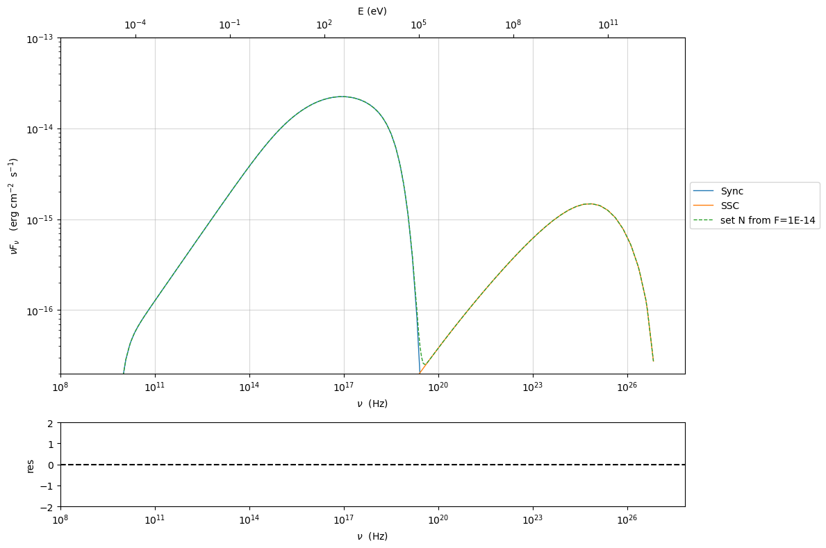
../../../../_images/Jet_example_phys_SSC_113_0.png

as you can see, the synchrotron flux at \(10^{15}\) Hz, now exactly matches the desired value of \(10^{-14}\) ergs cm-2 s-1. Alternatively, the value of N can be obtained using the rest-frame luminosity and frequency, using the method Jet.set_N_from_nuLnu()

my_jet.set_N_from_nuLnu(nuLnu_src=1E43,nu_src=1E15)

where nuLnu_src is the source rest-frame isotropic luminosity in erg/s at the rest-frame frequency nu_src in Hz.

Setting the beaming factor and expression#

Important

Starting from version 1.2.0, when using the delta expression, the value of delta used to compute jet luminosity will be set to beam_obj. In the previous versions, a reference value of 10 was used. In any case, if you are interested in evaluating jet luminosity you should use the beaming_expr method

It is possible to set the beaming factor according to the relativistic BulkFactor and viewing angle, this can be done by setting the beaming_expr kw in the Jet constructor, possible choices are

delta (default) to provide directly the beaming factor
bulk_theta to provide the BulkFactor and the jet viewing angle

my_jet=Jet(name='test',electron_distribution='lppl',beaming_expr='bulk_theta')

===> setting C threads to 12

my_jet.parameters.show_pars()

Table length=13

model name	name	par type	units	val	phys. bound. min	phys. bound. max	log	frozen
test	R	region_size	cm	5.000000e+15	1.000000e+03	1.000000e+30	False	False
test	R_H	region_position	cm	1.000000e+17	0.000000e+00	--	False	True
test	B	magnetic_field	gauss	1.000000e-01	0.000000e+00	--	False	False
test	NH_cold_to_rel_e	cold_p_to_rel_e_ratio		1.000000e+00	0.000000e+00	--	False	True
test	theta	jet-viewing-angle	deg	1.000000e-01	0.000000e+00	9.000000e+01	False	False
test	BulkFactor	jet-bulk-factor	lorentz-factor*	1.000000e+01	1.000000e+00	1.000000e+05	False	False
test	z_cosm	redshift		1.000000e-01	0.000000e+00	--	False	False
test	gmin	low-energy-cut-off	lorentz-factor*	2.000000e+00	1.000000e+00	1.000000e+09	False	False
test	gmax	high-energy-cut-off	lorentz-factor*	1.000000e+06	1.000000e+00	1.000000e+15	False	False
test	N	emitters_density	1 / cm3	1.000000e+02	0.000000e+00	--	False	False
test	gamma0_log_parab	turn-over-energy	lorentz-factor*	1.000000e+04	1.000000e+00	1.000000e+09	False	False
test	s	LE_spectral_slope		2.000000e+00	-1.000000e+01	1.000000e+01	False	False
test	r	spectral_curvature		4.000000e-01	-1.500000e+01	1.500000e+01	False	False

the actual value of the beaming factor can be obtained using the Jet.get_beaming()

my_jet.get_beaming()

19.94

We can change the value of theta and get the updated value of the beaming factor

my_jet.set_par('theta',val=10.)

my_jet.get_beaming()

4.968

of course setting beaming_expr=delta we get the same beaming expression as in the default case

my_jet=Jet(name='test',electron_distribution='lppl',beaming_expr='delta')

===> setting C threads to 12

my_jet.parameters.show_pars()

Table length=12

model name	name	par type	units	val	phys. bound. min	phys. bound. max	log	frozen
test	R	region_size	cm	5.000000e+15	1.000000e+03	1.000000e+30	False	False
test	R_H	region_position	cm	1.000000e+17	0.000000e+00	--	False	True
test	B	magnetic_field	gauss	1.000000e-01	0.000000e+00	--	False	False
test	NH_cold_to_rel_e	cold_p_to_rel_e_ratio		1.000000e+00	0.000000e+00	--	False	True
test	beam_obj	beaming		1.000000e+01	1.000000e-04	--	False	False
test	z_cosm	redshift		1.000000e-01	0.000000e+00	--	False	False
test	gmin	low-energy-cut-off	lorentz-factor*	2.000000e+00	1.000000e+00	1.000000e+09	False	False
test	gmax	high-energy-cut-off	lorentz-factor*	1.000000e+06	1.000000e+00	1.000000e+15	False	False
test	N	emitters_density	1 / cm3	1.000000e+02	0.000000e+00	--	False	False
test	gamma0_log_parab	turn-over-energy	lorentz-factor*	1.000000e+04	1.000000e+00	1.000000e+09	False	False
test	s	LE_spectral_slope		2.000000e+00	-1.000000e+01	1.000000e+01	False	False
test	r	spectral_curvature		4.000000e-01	-1.500000e+01	1.500000e+01	False	False

Switch ON/OFF Synchrotron sefl-absorption and IC emission#

my_jet.show_model()

--------------------------------------------------------------------------------
model description:
--------------------------------------------------------------------------------
type: Jet
name: test
geometry: spherical

electrons distribution:
 type: lppl
 gamma energy grid size:  201
 gmin grid : 2.000000e+00
 gmax grid : 1.000000e+06
 normalization:  True
 log-values:  False
 ratio of cold protons to relativistic electrons: 1.000000e+00

radiative fields:
 seed photons grid size:  100
 IC emission grid size:  100
 source emissivity lower bound :  1.000000e-120
 spectral components:
   name:Sum, state: on
   name:Sum, hidden: False
   name:Sync, state: self-abs
   name:Sync, hidden: False
   name:SSC, state: on
   name:SSC, hidden: False
external fields transformation method: blob

SED info:
 nu grid size jetkernel: 1000
 nu size: 500
 nu mix (Hz): 1.000000e+06
 nu max (Hz): 1.000000e+30

flux plot lower bound   :  1.000000e-30

--------------------------------------------------------------------------------

Table length=12

model name	name	par type	units	val	phys. bound. min	phys. bound. max	log	frozen
test	R	region_size	cm	5.000000e+15	1.000000e+03	1.000000e+30	False	False
test	R_H	region_position	cm	1.000000e+17	0.000000e+00	--	False	True
test	B	magnetic_field	gauss	1.000000e-01	0.000000e+00	--	False	False
test	NH_cold_to_rel_e	cold_p_to_rel_e_ratio		1.000000e+00	0.000000e+00	--	False	True
test	beam_obj	beaming		1.000000e+01	1.000000e-04	--	False	False
test	z_cosm	redshift		1.000000e-01	0.000000e+00	--	False	False
test	gmin	low-energy-cut-off	lorentz-factor*	2.000000e+00	1.000000e+00	1.000000e+09	False	False
test	gmax	high-energy-cut-off	lorentz-factor*	1.000000e+06	1.000000e+00	1.000000e+15	False	False
test	N	emitters_density	1 / cm3	1.000000e+02	0.000000e+00	--	False	False
test	gamma0_log_parab	turn-over-energy	lorentz-factor*	1.000000e+04	1.000000e+00	1.000000e+09	False	False
test	s	LE_spectral_slope		2.000000e+00	-1.000000e+01	1.000000e+01	False	False
test	r	spectral_curvature		4.000000e-01	-1.500000e+01	1.500000e+01	False	False

--------------------------------------------------------------------------------

as you see the state of Sync emission is self-abs, we can check accessing the specific spectral component state, and get the allowed states value

my_jet.spectral_components.Sync.show()

name                : Sync
var name            : do_Sync
state               : self-abs
allowed states : ['on', 'off', 'self-abs']

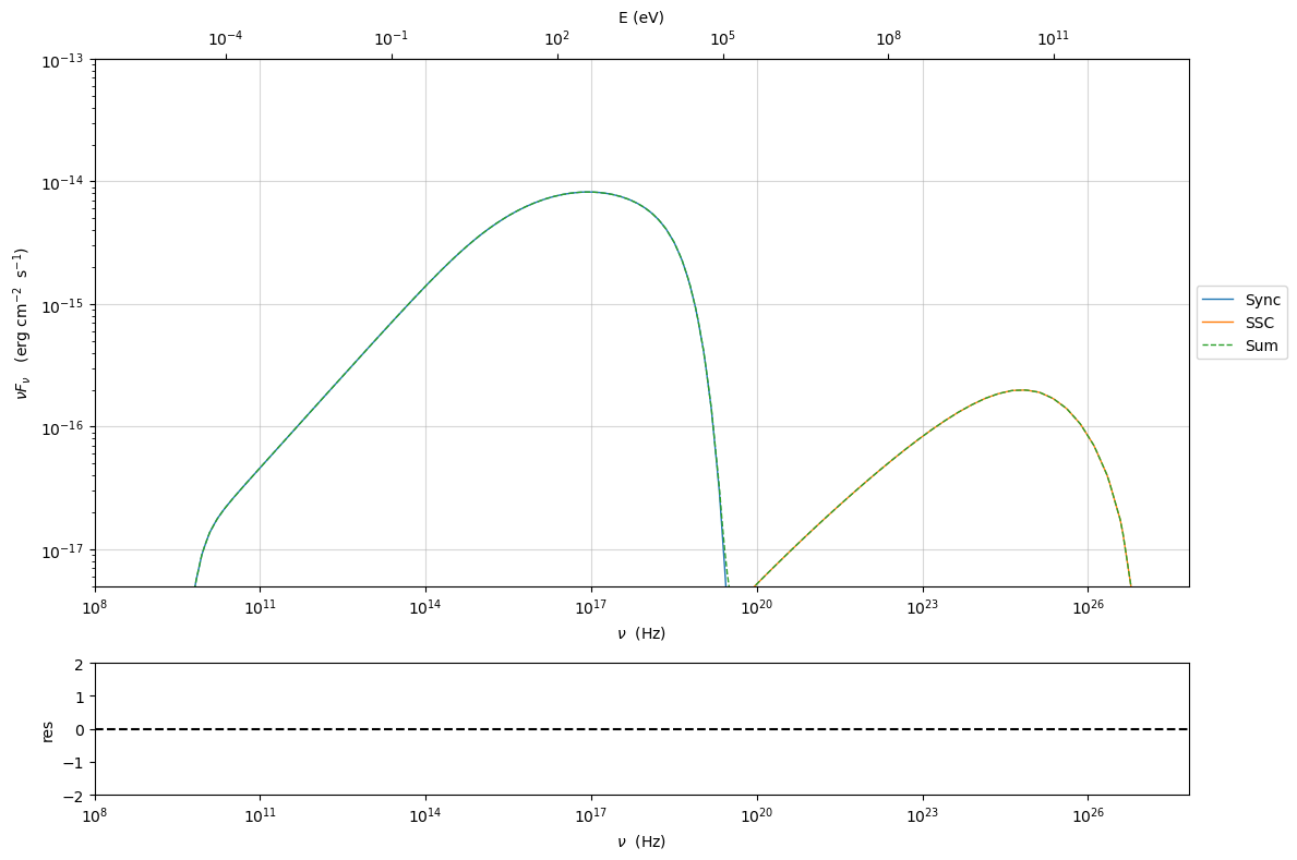
my_jet.spectral_components.Sync.state='on'

now the sate is ‘on’ with no ‘self-abs’

my_jet.eval()
p=my_jet.plot_model()
p.setlim(y_max=1E-13,y_min=5E-18,x_min=1E8)

../../../../_images/Jet_example_phys_SSC_136_0.png

to re-enable

my_jet.spectral_components.Sync.state='self-abs'
my_jet.eval()
p=my_jet.plot_model()
p.setlim(y_max=1E-13,y_min=5E-18,x_min=1E8)

../../../../_images/Jet_example_phys_SSC_138_0.png

my_jet.spectral_components.SSC.show()

name                : SSC
var name            : do_SSC
state               : on
allowed states : ['on', 'off']

my_jet.spectral_components.SSC.state='off'
my_jet.eval()
p=my_jet.plot_model()
p.setlim(y_max=1E-13,y_min=8E-18,x_min=1E8)

../../../../_images/Jet_example_phys_SSC_140_0.png

to re-enable

my_jet.spectral_components.SSC.state='on'
my_jet.eval()
p=my_jet.plot_model()
p.setlim(y_max=1E-13,y_min=8E-18,x_min=1E8)

../../../../_images/Jet_example_phys_SSC_142_0.png

Accessing individual spectral components#

It is possible to access specific spectral components of our model

my_jet=Jet(name='test',electron_distribution='lppl',beaming_expr='bulk_theta')
my_jet.eval()

===> setting C threads to 12

We can obtain this information anytime using the Jet.list_spectral_components() method

my_jet.list_spectral_components()

Sum
Sync
SSC

the on-screen message is telling us which components have been evaluated.

and we cann access a specific component using the Jet.get_spectral_component_by_name() method

Sync=my_jet.get_spectral_component_by_name('Sync')

Sync=my_jet.spectral_components.Sync

and from the SED object we can extract both the nu and nuFnu array

nu_sync=Sync.SED.nu
nuFnu_sync=Sync.SED.nuFnu

plt.loglog(nu_sync,nuFnu_sync)
plt.ylim(1E-20,1E-10)

(1e-20, 1e-10)

../../../../_images/Jet_example_phys_SSC_154_1.png

print (nuFnu_sync[::10])

[0.00000000e+00 0.00000000e+00 0.00000000e+00 6.04250670e-26
16351829e-24 9.84432972e-23 4.74613296e-21 2.28931297e-19
09662087e-17 1.83733916e-16 4.11135769e-16 7.21745036e-16
25581697e-15 2.18363181e-15 3.79383567e-15 6.57833387e-15
13501032e-14 1.93585563e-14 3.21429895e-14 5.06938061e-14
36908738e-14 9.77112603e-14 1.17645633e-13 1.28621805e-13
26850509e-13 1.10646286e-13 7.82537850e-14 3.17631756e-14
39710785e-15 8.88519981e-19 7.47780581e-29 0.00000000e+00
00000000e+00 0.00000000e+00 0.00000000e+00 0.00000000e+00
00000000e+00 0.00000000e+00 0.00000000e+00 0.00000000e+00
00000000e+00 0.00000000e+00 0.00000000e+00 0.00000000e+00
00000000e+00 0.00000000e+00 0.00000000e+00 0.00000000e+00
00000000e+00 0.00000000e+00] erg / (s cm2)

or for the src rest frame (isotropic luminosity)

nu_sync_src=Sync.SED.nu_src
nuLnu_sync_src=Sync.SED.nuLnu_src

print (nuLnu_sync_src[::10])

[0.00000000e+00 0.00000000e+00 0.00000000e+00 1.63219228e+30
84406112e+31 2.65913465e+33 1.28201787e+35 6.18385569e+36
96217481e+38 4.96299126e+39 1.11055338e+40 1.94956618e+40
39219277e+40 5.89839143e+40 1.02478484e+41 1.77692906e+41
06587177e+41 5.22910236e+41 8.68241307e+41 1.36933301e+42
99052613e+42 2.63936099e+42 3.17782509e+42 3.47431170e+42
42646573e+42 2.98875984e+42 2.11377876e+42 8.57981835e+41
47502951e+40 2.40005601e+37 2.01989298e+27 0.00000000e+00
00000000e+00 0.00000000e+00 0.00000000e+00 0.00000000e+00
00000000e+00 0.00000000e+00 0.00000000e+00 0.00000000e+00
00000000e+00 0.00000000e+00 0.00000000e+00 0.00000000e+00
00000000e+00 0.00000000e+00 0.00000000e+00 0.00000000e+00
00000000e+00 0.00000000e+00] erg / s

Moreover, you can access the corresponding astropy table

my_jet.spectral_components.build_table(restframe='obs')
t_obs=my_jet.spectral_components.table

t_obs[::10]

Table length=50

nu	Sum	Sync	SSC
Hz	erg / (s cm2)	erg / (s cm2)	erg / (s cm2)
float64	float64	float64	float64
1000000.0	0.0	0.0	0.0
3026648.059395689	0.0	0.0	0.0
9160598.47544371	0.0	0.0	0.0
27725907.59860481	6.042506698961876e-26	6.042506698961876e-26	0.0
83916564.42830162	2.163518310314854e-24	2.1635182921864927e-24	1.812816291990128e-32
253985906.87807292	9.844329807737109e-23	9.844329720868366e-23	8.68551689841149e-31
768725952.1663721	4.746132990060179e-21	4.746132957910235e-21	3.2149712394627884e-29
2326662911.331458	2.2893129865238557e-19	2.289312967845199e-19	1.8678480792336018e-27
7041989785.449296	1.0966208792227018e-17	1.0966208685756238e-17	1.064527310710398e-25
21313624718.414333	1.8373391925984397e-16	1.837339164979042e-16	2.7594342970944333e-24
64508840892.677124	4.1113579939584686e-16	4.111357687244127e-16	3.0649001085072766e-23
195245558101.6861	7.217452173223052e-16	7.21745035518903e-16	1.8173910289576096e-22
590939589534.0952	1.2558176489278755e-15	1.2558169671503148e-15	6.81696111297198e-22
1788566161883.4656	2.1836336700477045e-15	2.1836318098746114e-15	1.860089446152923e-21
5413360302965.376	3.793840076222717e-15	3.7938356685683746e-15	4.407555713355863e-21
16384336455779.848	6.578343589533983e-15	6.578333874972737e-15	9.71442266567319e-21
49589620138372.22	1.1350123615308075e-14	1.1350103170723414e-14	2.0444378457089687e-20
150090327557973.34	1.9358597962143978e-14	1.935855628475884e-14	4.1677039471748554e-20
454270598637404.3	3.214307262226785e-14	3.214298947301396e-14	8.31484748695644e-20
1374917225806420.5	5.069396875263241e-14	5.0693806110657886e-14	1.626398766134844e-19
4161390553316715.5	7.369118641741149e-14	7.369087378064904e-14	3.126306533382791e-19
1.2595064642583616e+16	9.771185152606807e-14	9.771126033092245e-14	5.9117995952915085e-19
...	...	...	...
9.682153059967095e+18	3.178273076119708e-14	3.17631756023561e-14	1.9547232856585933e-17
2.9304469769721385e+19	2.4307606323607617e-15	2.397107852227158e-15	3.3553024123860876e-17
8.869431656014668e+19	5.758868946575589e-17	8.885199812705549e-19	5.667587332078147e-17
2.6844648109619652e+20	9.407943419173862e-17	7.477805809126e-29	9.40794341916455e-17
8.124930210614097e+20	1.5343997652657038e-16	0.0	1.5343997652657038e-16
2.459130425468051e+21	2.459603692212681e-16	0.0	2.459603692212681e-16
7.442922330043758e+21	3.874834760928319e-16	0.0	3.874834760928319e-16
2.2527106426459734e+22	5.98977072597333e-16	0.0	5.98977072597333e-16
6.818162294944493e+22	9.050491218484525e-16	0.0	9.050491218484525e-16
2.0636177678638565e+23	1.328146971768062e-15	0.0	1.328146971768062e-15
6.245844712439592e+23	1.8718853701304056e-15	0.0	1.8718853701304056e-15
1.8903973778192233e+24	2.4815350094970205e-15	0.0	2.4815350094970205e-15
5.72156755506324e+24	2.9948879213537642e-15	0.0	2.9948879213537642e-15
1.7317171337233599e+25	3.1108073206153626e-15	0.0	3.1108073206153626e-15
5.2412983022060615e+25	2.583262880430937e-15	0.0	2.583262880430937e-15
1.5863565335085865e+26	1.5673161713761437e-15	0.0	1.5673161713761437e-15
4.801342923653465e+26	5.732736267795347e-16	0.0	5.732736267795347e-16
1.4531975242368953e+27	3.3493374925730033e-96	0.0	3.3493374925730033e-96
4.3983174666502106e+27	0.0	0.0	0.0
1.3312159025043105e+28	0.0	0.0	0.0
4.029122027951344e+28	0.0	0.0	0.0
1.2194734366967333e+29	0.0	0.0	0.0
3.690916910662782e+29	0.0	0.0	0.0

and also in the src restframe

my_jet.spectral_components.build_table(restframe='src')
t_src=my_jet.spectral_components.table

t_src[::10]

Table length=50

nu	Sum	Sync	SSC
Hz	erg / s	erg / s	erg / s
float64	float64	float64	float64
1100000.0	0.0	0.0	0.0
3329312.865335258	0.0	0.0	0.0
10076658.322988082	0.0	0.0	0.0
30498498.35846529	1.6321922754264707e+30	1.6321922754264707e+30	0.0
92308220.8711318	5.84406116495712e+31	5.84406111598908e+31	4.896750464607491e+23
279384497.56588024	2.6591346719896186e+33	2.659134648524772e+33	2.3461179765193927e+25
845598547.3830093	1.2820178760999728e+35	1.2820178674156813e+35	8.684229052937516e+26
2559329202.464604	6.183855738678291e+36	6.183855688223801e+36	5.045401450889629e+28
7746188763.994226	2.9621748345702107e+38	2.9621748058104933e+38	2.875484199000618e+30
23444987190.255768	4.962991332740602e+39	4.962991258135525e+39	7.453739927236154e+31
70959724981.94484	1.1105534662302938e+40	1.110553383381105e+40	8.278859306715832e+32
214770113911.85474	1.9495666736155294e+40	1.9495661825310782e+40	4.9091076711650177e+33
650033548487.5048	3.392194610684439e+40	3.3921927690777626e+40	1.841386666958448e+34
1967422778071.8123	5.898396453950717e+40	5.898391429280816e+40	5.024443954914775e+34
5954696333261.914	1.0247860325381098e+41	1.0247848419495463e+41	1.1905619219399787e+35
18022770101357.832	1.7769316819761714e+41	1.776929057894376e+41	2.6240443618976355e+35
54548582152209.445	3.065877294471873e+41	3.065871772013261e+41	5.5224029125677384e+35
165099360313770.7	5.229113616427845e+41	5.229102358599022e+41	1.1257735452758212e+36
499697658501144.8	8.682435528213993e+41	8.682413068070106e+41	2.2459933460878286e+36
1512408948387062.8	1.3693374013631282e+42	1.3693330081040437e+42	4.393202415984916e+36
4577529608648387.0	1.990534578276517e+42	1.9905261333821364e+42	8.444729362533213e+36
1.3854571106841978e+16	2.639376954366745e+42	2.6393609850977307e+42	1.5968858809808022e+37
...	...	...	...
1.0650368365963805e+19	8.585100559226115e+41	8.579818350898489e+41	5.2800673733573894e+38
3.2234916746693526e+19	6.5659318643893655e+40	6.475029511248192e+40	9.06328937981526e+38
9.756374821616135e+19	1.5555764979803717e+39	2.4000560069565626e+37	1.5309196538105874e+39
2.952911292058162e+20	2.5412586764799147e+39	2.019892982641053e+27	2.5412586764773993e+39
8.937423231675508e+20	4.1446961816577584e+39	0.0	4.1446961816577584e+39
2.7050434680148564e+21	6.643842277791231e+39	0.0	6.643842277791231e+39
8.187214563048134e+21	1.0466641876338746e+40	0.0	1.0466641876338746e+40
2.477981706910571e+22	1.6179473184843802e+40	0.0	1.6179473184843802e+40
7.499978524438943e+22	2.4447042579470295e+40	0.0	2.4447042579470295e+40
2.2699795446502424e+23	3.5875694243306733e+40	0.0	3.5875694243306733e+40
6.870429183683552e+23	5.056306916690014e+40	0.0	5.056306916690014e+40
2.0794371156011458e+24	6.703082802369509e+40	0.0	6.703082802369509e+40
6.293724310569564e+24	8.08974350304232e+40	0.0	8.08974350304232e+40
1.904888847095696e+25	8.402863136123344e+40	0.0	8.402863136123344e+40
5.765428132426668e+25	6.977868505399752e+40	0.0	6.977868505399752e+40
1.744992186859445e+26	4.2336094530282163e+40	0.0	4.2336094530282163e+40
5.2814772160188116e+26	1.5485175804538692e+40	0.0	1.5485175804538692e+40
1.598517276660585e+27	9.047177033520093e-41	0.0	9.047177033520093e-41
4.838149213315232e+27	0.0	0.0	0.0
1.4643374927547416e+28	0.0	0.0	0.0
4.432034230746478e+28	0.0	0.0	0.0
1.3414207803664067e+29	0.0	0.0	0.0
4.060008601729061e+29	0.0	0.0	0.0

Of cousrse, since these colums have units, you can easily convert the units of the Synchrotron luminostity form erg/s to GeV/s

t_src['Sync'][::10].to('GeV/s')

\[[0,~0,~0,~1.0187343 \times 10^{33},~3.647576 \times 10^{34},~1.6597013 \times 10^{36},~8.0017262 \times 10^{37},~3.8596591 \times 10^{39},~1.8488441 \times 10^{41},~3.0976555 \times 10^{42},~6.931529 \times 10^{42},~1.2168235 \times 10^{43},~2.1172402 \times 10^{43},~3.6814864 \times 10^{43},~6.3962039 \times 10^{43},~1.1090719 \times 10^{44},~1.9135666 \times 10^{44},~3.263749 \times 10^{44},~5.419136 \times 10^{44},~8.5467044 \times 10^{44},~1.2423887 \times 10^{45},~1.6473596 \times 10^{45},~1.9834424 \times 10^{45},~2.1684948 \times 10^{45},~2.1386317 \times 10^{45},~1.8654372 \times 10^{45},~1.3193169 \times 10^{45},~5.3551014 \times 10^{44},~4.0413955 \times 10^{43},~1.4979971 \times 10^{40},~1.260718 \times 10^{30},~0,~0,~0,~0,~0,~0,~0,~0,~0,~0,~0,~0,~0,~0,~0,~0,~0,~0,~0] \; \mathrm{\frac{GeV}{s}}\]

the table can be easily saved as an ascii file

t_src.write('test_SED.txt',format='ascii.ecsv',overwrite=True)

or in fits format

t_src.write('test_SED.fits',format='fits',overwrite=True)

WARNING: VerifyWarning: Keyword name 'model_name' is greater than 8 characters or contains characters not allowed by the FITS standard; a HIERARCH card will be created. [astropy.io.fits.card]
WARNING: VerifyWarning: Keyword name 'restframe' is greater than 8 characters or contains characters not allowed by the FITS standard; a HIERARCH card will be created. [astropy.io.fits.card]

Energetic report#

It is possible to get an energetic report of the jet model (updated each time that you evaluate the model). This report gives energy densities (U_) (both in the blob end disk restframe), the luminosities of the emitted components in the blob restframe (L_), and the luminosity carried by the jet (jet_L) for the radiative components, the electrons, the magnetic fields, and for the cold protons in the jet.

case of beaming expression ‘bulk_theta’#

Note

In this case, the BulkFactor used for the energetic report will be the one taken from the jet parameters, in this case we set BulkFactor=15

my_jet=Jet(name='test',electron_distribution='lppl',beaming_expr='bulk_theta')
my_jet.parameters.BulkFactor.val=15

===> setting C threads to 12

my_jet

--------------------------------------------------------------------------------
model description:
--------------------------------------------------------------------------------
type: Jet
name: test
geometry: spherical

electrons distribution:
 type: lppl
 gamma energy grid size:  201
 gmin grid : 2.000000e+00
 gmax grid : 1.000000e+06
 normalization:  True
 log-values:  False
 ratio of cold protons to relativistic electrons: 1.000000e+00

radiative fields:
 seed photons grid size:  100
 IC emission grid size:  100
 source emissivity lower bound :  1.000000e-120
 spectral components:
   name:Sum, state: on
   name:Sum, hidden: False
   name:Sync, state: self-abs
   name:Sync, hidden: False
   name:SSC, state: on
   name:SSC, hidden: False
external fields transformation method: blob

SED info:
 nu grid size jetkernel: 1000
 nu size: 500
 nu mix (Hz): 1.000000e+06
 nu max (Hz): 1.000000e+30

flux plot lower bound   :  1.000000e-30

--------------------------------------------------------------------------------

Table length=13

model name	name	par type	units	val	phys. bound. min	phys. bound. max	log	frozen
test	R	region_size	cm	5.000000e+15	1.000000e+03	1.000000e+30	False	False
test	R_H	region_position	cm	1.000000e+17	0.000000e+00	--	False	True
test	B	magnetic_field	gauss	1.000000e-01	0.000000e+00	--	False	False
test	NH_cold_to_rel_e	cold_p_to_rel_e_ratio		1.000000e+00	0.000000e+00	--	False	True
test	theta	jet-viewing-angle	deg	1.000000e-01	0.000000e+00	9.000000e+01	False	False
test	BulkFactor	jet-bulk-factor	lorentz-factor*	1.500000e+01	1.000000e+00	1.000000e+05	False	False
test	z_cosm	redshift		1.000000e-01	0.000000e+00	--	False	False
test	gmin	low-energy-cut-off	lorentz-factor*	2.000000e+00	1.000000e+00	1.000000e+09	False	False
test	gmax	high-energy-cut-off	lorentz-factor*	1.000000e+06	1.000000e+00	1.000000e+15	False	False
test	N	emitters_density	1 / cm3	1.000000e+02	0.000000e+00	--	False	False
test	gamma0_log_parab	turn-over-energy	lorentz-factor*	1.000000e+04	1.000000e+00	1.000000e+09	False	False
test	s	LE_spectral_slope		2.000000e+00	-1.000000e+01	1.000000e+01	False	False
test	r	spectral_curvature		4.000000e-01	-1.500000e+01	1.500000e+01	False	False

--------------------------------------------------------------------------------

None

my_jet.eval()

my_jet.energetic_report()

Table length=39

name	type	units	val
BulkLorentzFactor	jet-bulk-factor		1.500000e+01
U_e	Energy dens. blob rest. frame	erg / cm3	1.736635e-03
U_p_cold	Energy dens. blob rest. frame	erg / cm3	1.503276e-01
U_B	Energy dens. blob rest. frame	erg / cm3	3.978874e-04
U_Synch	Energy dens. blob rest. frame	erg / cm3	1.831568e-05
U_Synch_DRF	Energy dens. disk rest. frame	erg / cm3	1.472951e+01
U_Disk	Energy dens. blob rest. frame	erg / cm3	0.000000e+00
U_BLR	Energy dens. blob rest. frame	erg / cm3	0.000000e+00
U_DT	Energy dens. blob rest. frame	erg / cm3	0.000000e+00
U_CMB	Energy dens. blob rest. frame	erg / cm3	0.000000e+00
U_Star	Energy dens. blob rest. frame	erg / cm3	0.000000e+00
U_Disk_DRF	Energy dens. disk rest. frame	erg / cm3	0.000000e+00
U_BLR_DRF	Energy dens. disk rest. frame	erg / cm3	0.000000e+00
U_DT_DRF	Energy dens. disk rest. frame	erg / cm3	0.000000e+00
U_CMB_DRF	Energy dens. disk rest. frame	erg / cm3	0.000000e+00
U_Star_DRF	Energy dens. disk rest. frame	erg / cm3	0.000000e+00
U_seed_tot	Energy dens. blob rest. frame	erg / cm3	1.831568e-05
L_Sync_rf	Lum. blob rest. frame.	erg / s	1.725018e+38
L_SSC_rf	Lum. blob rest. frame.	erg / s	3.823311e+36
L_EC_Disk_rf	Lum. blob rest. frame.	erg / s	0.000000e+00
L_EC_BLR_rf	Lum. blob rest. frame.	erg / s	0.000000e+00
L_EC_DT_rf	Lum. blob rest. frame.	erg / s	0.000000e+00
L_EC_CMB_rf	Lum. blob rest. frame.	erg / s	0.000000e+00
L_EC_Star_rf	Lum. blob rest. frame.	erg / s	0.000000e+00
jet_L_Sync	jet Lum.	erg / s	9.681638e+39
jet_L_SSC	jet Lum.	erg / s	2.145828e+38
jet_L_EC_Disk	jet Lum.	erg / s	0.000000e+00
jet_L_EC_BLR	jet Lum.	erg / s	0.000000e+00
jet_L_EC_Star	jet Lum.	erg / s	0.000000e+00
jet_L_EC_DT	jet Lum.	erg / s	0.000000e+00
jet_L_EC_CMB	jet Lum.	erg / s	0.000000e+00
jet_L_pp_gamma	jet Lum.	erg / s	0.000000e+00
jet_L_rad	jet Lum.	erg / s	9.896221e+39
jet_L_kin	jet Lum.	erg / s	8.038094e+43
jet_L_tot	jet Lum.	erg / s	8.060115e+43
jet_L_e	jet Lum.	erg / s	9.179824e+41
jet_L_B	jet Lum.	erg / s	2.103226e+41
jet_L_p_cold	jet Lum.	erg / s	7.946295e+43
NH_cold_to_rel_e	cold_p_to_rel_e_ratio		1.000000e+00

Note

NH_cold_to_rel_e represents the ratio of cold protons to relativistic electrons used to compute the cold protons energetic

If you want to evaluate the energetic report in non verbose mode:

my_jet.energetic_report(verbose=False)

my_jet.energetic_dict

{'BulkLorentzFactor': 15,
 'U_e': 0.001737,
 'U_p_cold': 0.1503,
 'U_B': 0.0003979,
 'U_Synch': 1.832e-05,
 'U_Synch_DRF': 14.73,
 'U_Disk': 0,
 'U_BLR': 0,
 'U_DT': 0,
 'U_CMB': 0,
 'U_Star': 0,
 'U_Disk_DRF': 0,
 'U_BLR_DRF': 0,
 'U_DT_DRF': 0,
 'U_CMB_DRF': 0,
 'U_Star_DRF': 0,
 'U_seed_tot': 1.832e-05,
 'L_Sync_rf': 1.725e+38,
 'L_SSC_rf': 3.823e+36,
 'L_EC_Disk_rf': 0,
 'L_EC_BLR_rf': 0,
 'L_EC_DT_rf': 0,
 'L_EC_CMB_rf': 0,
 'L_EC_Star_rf': 0,
 'jet_L_Sync': 9.682e+39,
 'jet_L_SSC': 2.146e+38,
 'jet_L_EC_Disk': 0,
 'jet_L_EC_BLR': 0,
 'jet_L_EC_Star': 0,
 'jet_L_EC_DT': 0,
 'jet_L_EC_CMB': 0,
 'jet_L_pp_gamma': 0,
 'jet_L_rad': 9.896e+39,
 'jet_L_kin': 8.038e+43,
 'jet_L_tot': 8.06e+43,
 'jet_L_e': 9.18e+41,
 'jet_L_B': 2.103e+41,
 'jet_L_p_cold': 7.946e+43,
 'NH_cold_to_rel_e': 1}

my_jet.energetic_report_table

Table length=39

name	type	units	val
str17	str29	object	float64
BulkLorentzFactor	jet-bulk-factor		1.500000e+01
U_e	Energy dens. blob rest. frame	erg / cm3	1.736635e-03
U_p_cold	Energy dens. blob rest. frame	erg / cm3	1.503276e-01
U_B	Energy dens. blob rest. frame	erg / cm3	3.978874e-04
U_Synch	Energy dens. blob rest. frame	erg / cm3	1.831568e-05
U_Synch_DRF	Energy dens. disk rest. frame	erg / cm3	1.472951e+01
U_Disk	Energy dens. blob rest. frame	erg / cm3	0.000000e+00
U_BLR	Energy dens. blob rest. frame	erg / cm3	0.000000e+00
U_DT	Energy dens. blob rest. frame	erg / cm3	0.000000e+00
U_CMB	Energy dens. blob rest. frame	erg / cm3	0.000000e+00
U_Star	Energy dens. blob rest. frame	erg / cm3	0.000000e+00
U_Disk_DRF	Energy dens. disk rest. frame	erg / cm3	0.000000e+00
U_BLR_DRF	Energy dens. disk rest. frame	erg / cm3	0.000000e+00
U_DT_DRF	Energy dens. disk rest. frame	erg / cm3	0.000000e+00
U_CMB_DRF	Energy dens. disk rest. frame	erg / cm3	0.000000e+00
U_Star_DRF	Energy dens. disk rest. frame	erg / cm3	0.000000e+00
U_seed_tot	Energy dens. blob rest. frame	erg / cm3	1.831568e-05
L_Sync_rf	Lum. blob rest. frame.	erg / s	1.725018e+38
L_SSC_rf	Lum. blob rest. frame.	erg / s	3.823311e+36
L_EC_Disk_rf	Lum. blob rest. frame.	erg / s	0.000000e+00
L_EC_BLR_rf	Lum. blob rest. frame.	erg / s	0.000000e+00
L_EC_DT_rf	Lum. blob rest. frame.	erg / s	0.000000e+00
L_EC_CMB_rf	Lum. blob rest. frame.	erg / s	0.000000e+00
L_EC_Star_rf	Lum. blob rest. frame.	erg / s	0.000000e+00
jet_L_Sync	jet Lum.	erg / s	9.681638e+39
jet_L_SSC	jet Lum.	erg / s	2.145828e+38
jet_L_EC_Disk	jet Lum.	erg / s	0.000000e+00
jet_L_EC_BLR	jet Lum.	erg / s	0.000000e+00
jet_L_EC_Star	jet Lum.	erg / s	0.000000e+00
jet_L_EC_DT	jet Lum.	erg / s	0.000000e+00
jet_L_EC_CMB	jet Lum.	erg / s	0.000000e+00
jet_L_pp_gamma	jet Lum.	erg / s	0.000000e+00
jet_L_rad	jet Lum.	erg / s	9.896221e+39
jet_L_kin	jet Lum.	erg / s	8.038094e+43
jet_L_tot	jet Lum.	erg / s	8.060115e+43
jet_L_e	jet Lum.	erg / s	9.179824e+41
jet_L_B	jet Lum.	erg / s	2.103226e+41
jet_L_p_cold	jet Lum.	erg / s	7.946295e+43
NH_cold_to_rel_e	cold_p_to_rel_e_ratio		1.000000e+00

my_jet.show_model()

--------------------------------------------------------------------------------
model description:
--------------------------------------------------------------------------------
type: Jet
name: test
geometry: spherical

electrons distribution:
 type: lppl
 gamma energy grid size:  201
 gmin grid : 2.000000e+00
 gmax grid : 1.000000e+06
 normalization:  True
 log-values:  False
 ratio of cold protons to relativistic electrons: 1.000000e+00

radiative fields:
 seed photons grid size:  100
 IC emission grid size:  100
 source emissivity lower bound :  1.000000e-120
 spectral components:
   name:Sum, state: on
   name:Sum, hidden: False
   name:Sync, state: self-abs
   name:Sync, hidden: False
   name:SSC, state: on
   name:SSC, hidden: False
external fields transformation method: blob

SED info:
 nu grid size jetkernel: 1000
 nu size: 500
 nu mix (Hz): 1.000000e+06
 nu max (Hz): 1.000000e+30

flux plot lower bound   :  1.000000e-30

--------------------------------------------------------------------------------

Table length=13

model name	name	par type	units	val	phys. bound. min	phys. bound. max	log	frozen
test	R	region_size	cm	5.000000e+15	1.000000e+03	1.000000e+30	False	False
test	R_H	region_position	cm	1.000000e+17	0.000000e+00	--	False	True
test	B	magnetic_field	gauss	1.000000e-01	0.000000e+00	--	False	False
test	NH_cold_to_rel_e	cold_p_to_rel_e_ratio		1.000000e+00	0.000000e+00	--	False	True
test	theta	jet-viewing-angle	deg	1.000000e-01	0.000000e+00	9.000000e+01	False	False
test	BulkFactor	jet-bulk-factor	lorentz-factor*	1.500000e+01	1.000000e+00	1.000000e+05	False	False
test	z_cosm	redshift		1.000000e-01	0.000000e+00	--	False	False
test	gmin	low-energy-cut-off	lorentz-factor*	2.000000e+00	1.000000e+00	1.000000e+09	False	False
test	gmax	high-energy-cut-off	lorentz-factor*	1.000000e+06	1.000000e+00	1.000000e+15	False	False
test	N	emitters_density	1 / cm3	1.000000e+02	0.000000e+00	--	False	False
test	gamma0_log_parab	turn-over-energy	lorentz-factor*	1.000000e+04	1.000000e+00	1.000000e+09	False	False
test	s	LE_spectral_slope		2.000000e+00	-1.000000e+01	1.000000e+01	False	False
test	r	spectral_curvature		4.000000e-01	-1.500000e+01	1.500000e+01	False	False

--------------------------------------------------------------------------------

case of beaming expression ‘delta’#

Note

In this case, the BulkFactor used for the energetic report will be the beaming factor parameter beam_obj

my_jet=Jet(name='test',electron_distribution='lppl',beaming_expr='delta')
my_jet.parameters.beam_obj.val=25
my_jet.eval()

===> setting C threads to 12

my_jet.energetic_report()

Table length=39

name	type	units	val
BulkLorentzFactor	jet-bulk-factor		2.500000e+01
U_e	Energy dens. blob rest. frame	erg / cm3	1.736635e-03
U_p_cold	Energy dens. blob rest. frame	erg / cm3	1.503276e-01
U_B	Energy dens. blob rest. frame	erg / cm3	3.978874e-04
U_Synch	Energy dens. blob rest. frame	erg / cm3	1.831568e-05
U_Synch_DRF	Energy dens. disk rest. frame	erg / cm3	7.154561e+00
U_Disk	Energy dens. blob rest. frame	erg / cm3	0.000000e+00
U_BLR	Energy dens. blob rest. frame	erg / cm3	0.000000e+00
U_DT	Energy dens. blob rest. frame	erg / cm3	0.000000e+00
U_CMB	Energy dens. blob rest. frame	erg / cm3	0.000000e+00
U_Star	Energy dens. blob rest. frame	erg / cm3	0.000000e+00
U_Disk_DRF	Energy dens. disk rest. frame	erg / cm3	0.000000e+00
U_BLR_DRF	Energy dens. disk rest. frame	erg / cm3	0.000000e+00
U_DT_DRF	Energy dens. disk rest. frame	erg / cm3	0.000000e+00
U_CMB_DRF	Energy dens. disk rest. frame	erg / cm3	0.000000e+00
U_Star_DRF	Energy dens. disk rest. frame	erg / cm3	0.000000e+00
U_seed_tot	Energy dens. blob rest. frame	erg / cm3	1.831568e-05
L_Sync_rf	Lum. blob rest. frame.	erg / s	1.725018e+38
L_SSC_rf	Lum. blob rest. frame.	erg / s	3.823311e+36
L_EC_Disk_rf	Lum. blob rest. frame.	erg / s	0.000000e+00
L_EC_BLR_rf	Lum. blob rest. frame.	erg / s	0.000000e+00
L_EC_DT_rf	Lum. blob rest. frame.	erg / s	0.000000e+00
L_EC_CMB_rf	Lum. blob rest. frame.	erg / s	0.000000e+00
L_EC_Star_rf	Lum. blob rest. frame.	erg / s	0.000000e+00
jet_L_Sync	jet Lum.	erg / s	2.693183e+40
jet_L_SSC	jet Lum.	erg / s	5.969143e+38
jet_L_EC_Disk	jet Lum.	erg / s	0.000000e+00
jet_L_EC_BLR	jet Lum.	erg / s	0.000000e+00
jet_L_EC_Star	jet Lum.	erg / s	0.000000e+00
jet_L_EC_DT	jet Lum.	erg / s	0.000000e+00
jet_L_EC_CMB	jet Lum.	erg / s	0.000000e+00
jet_L_pp_gamma	jet Lum.	erg / s	0.000000e+00
jet_L_rad	jet Lum.	erg / s	2.752874e+40
jet_L_kin	jet Lum.	erg / s	2.235991e+44
jet_L_tot	jet Lum.	erg / s	2.242117e+44
jet_L_e	jet Lum.	erg / s	2.553591e+42
jet_L_B	jet Lum.	erg / s	5.850635e+41
jet_L_p_cold	jet Lum.	erg / s	2.210455e+44
NH_cold_to_rel_e	cold_p_to_rel_e_ratio		1.000000e+00

Physical setup

Contents

Physical setup#

Basic setup and C threads#

C threads#

basic configurations#

Setting the parameters#

Investigating the electron distribution#

Using log values for electron distribution parameters#

Evaluate and plot the model#

Changing the nu grid#

Comparing models on the same plot#

Saving a plot#

Saving and loading a model#

Switching on/off the particle distribution normalization#

Setting the particle density from observed Fluxes or Luminosities#

Setting the beaming factor and expression#

Switch ON/OFF Synchrotron sefl-absorption and IC emission#

Accessing individual spectral components#

Energetic report#

case of beaming expression ‘bulk_theta’#

case of beaming expression ‘delta’#