Model fitting 1: Only SSC#

import warnings
warnings.filterwarnings('ignore')

import matplotlib.pylab as plt
import jetset
from jetset.test_data_helper import  test_SEDs
from jetset.data_loader import ObsData,Data
from jetset.plot_sedfit import PlotSED
from jetset.test_data_helper import  test_SEDs

print(jetset.__version__)

1.3.0rc7

test_SEDs

['/Users/orion/miniforge3/envs/jetset/lib/python3.10/site-packages/jetset/test_data/SEDs_data/SED_3C345.ecsv',
 '/Users/orion/miniforge3/envs/jetset/lib/python3.10/site-packages/jetset/test_data/SEDs_data/SED_MW_Mrk421_EBL_DEABS.ecsv',
 '/Users/orion/miniforge3/envs/jetset/lib/python3.10/site-packages/jetset/test_data/SEDs_data/SED_MW_Mrk501_EBL_ABS.ecsv',
 '/Users/orion/miniforge3/envs/jetset/lib/python3.10/site-packages/jetset/test_data/SEDs_data/SED_MW_Mrk501_EBL_DEABS.ecsv']

Loading data#

see the Data format and SED data user guide for further information about loading data

print(test_SEDs[1])
data=Data.from_file(test_SEDs[1])

/Users/orion/miniforge3/envs/jetset/lib/python3.10/site-packages/jetset/test_data/SEDs_data/SED_MW_Mrk421_EBL_DEABS.ecsv

%matplotlib inline
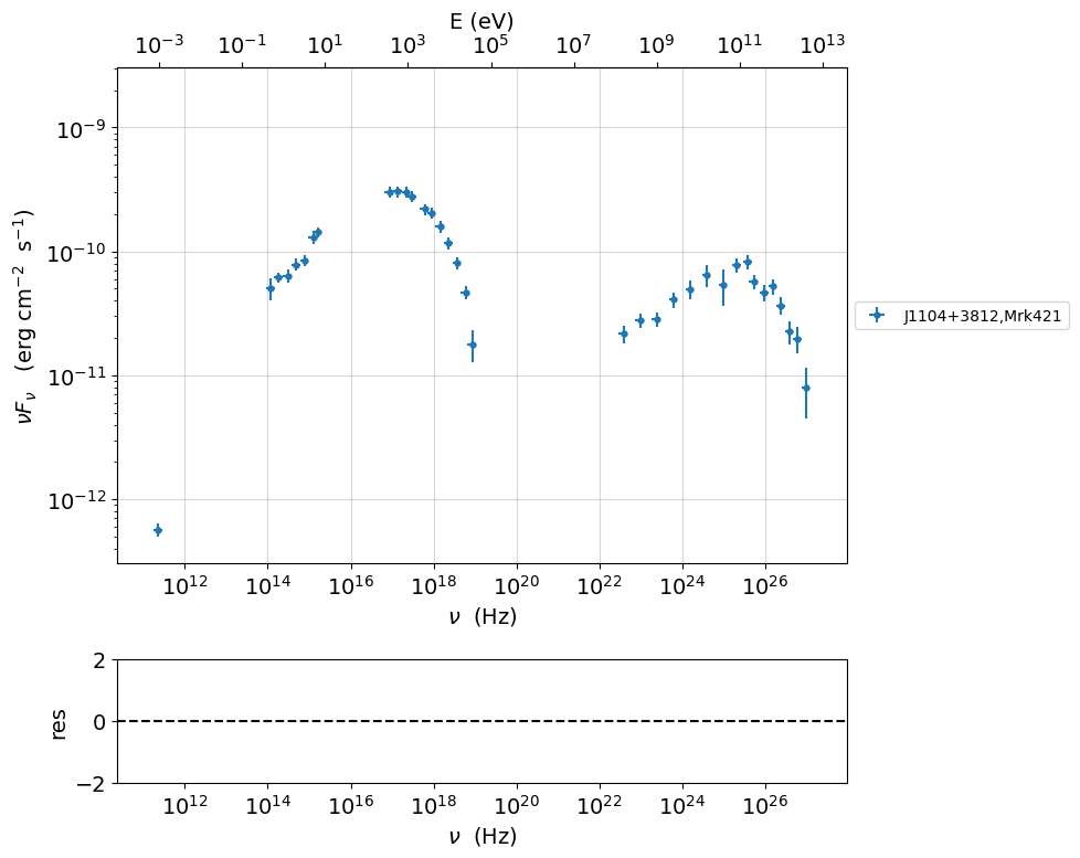
sed_data=ObsData(data_table=data)
sed_data.group_data(bin_width=0.2)

sed_data.add_systematics(0.1,[10.**6,10.**29])
p=sed_data.plot_sed()
#p.setlim(y_min=1E-15,x_min=1E7,x_max=1E29)

================================================================================

*  binning data  *
---> N bins= 89
---> bin_widht= 0.2
msk [False  True False  True  True  True  True  True False False False  True
 False False False False False False False False False False False False
  True  True  True  True  True  True  True False False False False False
 False False  True  True  True  True  True  True  True  True  True  True
  True False False False False False False False False False False False
 False False False False False False  True False  True False  True False
  True  True False  True False  True False  True  True  True  True  True
  True  True  True  True False]
================================================================================

../../../../_images/Jet_example_model_fit_8_1.png

sed_data.save('Mrk_401.pkl')

phenomenological model constraining#

see the Phenomenological model constraining: application user guide for further information about phenomenological constraining

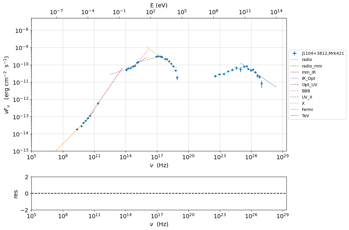
spectral indices#

from jetset.sed_shaper import  SEDShape
my_shape=SEDShape(sed_data)
my_shape.eval_indices(minimizer='lsb',silent=True)
p=my_shape.plot_indices()
p.setlim(y_min=1E-15,y_max=5E-8)

================================================================================

* evaluating spectral indices for data *
================================================================================

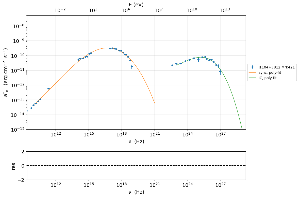
../../../../_images/Jet_example_model_fit_13_1.png

sed shaper#

mm,best_fit=my_shape.sync_fit(check_host_gal_template=False,
                  Ep_start=None,
                  minimizer='lsb',
                  silent=True,
                  fit_range=[10.,21.])

================================================================================

* Log-Polynomial fitting of the synchrotron component *
---> first blind fit run,  fit range: [10.0, 21.0]
---> class:  HSP

Table length=4

model name	name	val	bestfit val	err +	err -	start val	fit range min	fit range max	frozen
LogCubic	b	-1.585748e-01	-1.585748e-01	6.470535e-03	--	-1.000000e+00	-1.000000e+01	0.000000e+00	False
LogCubic	c	-1.089513e-02	-1.089513e-02	9.764985e-04	--	-1.000000e+00	-1.000000e+01	1.000000e+01	False
LogCubic	Ep	1.673177e+01	1.673177e+01	2.478677e-02	--	1.667298e+01	0.000000e+00	3.000000e+01	False
LogCubic	Sp	-9.489417e+00	-9.489417e+00	1.853260e-02	--	-1.000000e+01	-3.000000e+01	0.000000e+00	False

---> sync       nu_p=+1.673177e+01 (err=+2.478677e-02)  nuFnu_p=-9.489417e+00 (err=+1.853260e-02) curv.=-1.585748e-01 (err=+6.470535e-03)
================================================================================

my_shape.IC_fit(fit_range=[23.,29.],minimizer='minuit',silent=True)
p=my_shape.plot_shape_fit()
p.setlim(y_min=1E-15,y_max=5E-8)

================================================================================

* Log-Polynomial fitting of the IC component *
---> fit range: [23.0, 29.0]
---> LogCubic fit
====> simplex
====> migrad
====> simplex
====> migrad
====> simplex
====> migrad

Table length=4

model name	name	val	bestfit val	err +	err -	start val	fit range min	fit range max	frozen
LogCubic	b	-1.971111e-01	-1.971111e-01	2.679732e-02	--	-1.000000e+00	-1.000000e+01	0.000000e+00	False
LogCubic	c	-4.037544e-02	-4.037544e-02	2.119803e-02	--	-1.000000e+00	-1.000000e+01	1.000000e+01	False
LogCubic	Ep	2.521789e+01	2.521789e+01	1.198160e-01	--	2.529262e+01	0.000000e+00	3.000000e+01	False
LogCubic	Sp	-1.012535e+01	-1.012535e+01	2.996508e-02	--	-1.000000e+01	-3.000000e+01	0.000000e+00	False

---> IC         nu_p=+2.521789e+01 (err=+1.198160e-01)  nuFnu_p=-1.012535e+01 (err=+2.996508e-02) curv.=-1.971111e-01 (err=+2.679732e-02)
================================================================================

../../../../_images/Jet_example_model_fit_16_3.png

Model constraining#

In this step we are not fitting the model, we are just obtaining the phenomenological pre_fit model, that will be fitted in using minuit ore least-square bound, as shown below

from jetset.obs_constrain import ObsConstrain
from jetset.model_manager import  FitModel
sed_obspar=ObsConstrain(beaming=25,
                        B_range=[0.001,0.1],
                        distr_e='lppl',
                        t_var_sec=3*86400,
                        nu_cut_IR=1E12,
                        SEDShape=my_shape)


prefit_jet=sed_obspar.constrain_SSC_model(electron_distribution_log_values=False,silent=True)
prefit_jet.save_model('prefit_jet.pkl')

================================================================================

*  constrains parameters from observable *

===> setting C threads to 12

Table length=12

model name	name	par type	units	val	phys. bound. min	phys. bound. max	log	frozen
jet_leptonic	R	region_size	cm	3.460321e+16	1.000000e+03	1.000000e+30	False	False
jet_leptonic	R_H	region_position	cm	1.000000e+17	0.000000e+00	--	False	True
jet_leptonic	B	magnetic_field	gauss	5.050000e-02	0.000000e+00	--	False	False
jet_leptonic	NH_cold_to_rel_e	cold_p_to_rel_e_ratio		1.000000e+00	0.000000e+00	--	False	True
jet_leptonic	beam_obj	beaming		2.500000e+01	1.000000e-04	--	False	False
jet_leptonic	z_cosm	redshift		3.080000e-02	0.000000e+00	--	False	False
jet_leptonic	gmin	low-energy-cut-off	lorentz-factor*	4.697542e+02	1.000000e+00	1.000000e+09	False	False
jet_leptonic	gmax	high-energy-cut-off	lorentz-factor*	1.373160e+06	1.000000e+00	1.000000e+15	False	False
jet_leptonic	N	emitters_density	1 / cm3	6.545152e-01	0.000000e+00	--	False	False
jet_leptonic	gamma0_log_parab	turn-over-energy	lorentz-factor*	3.333017e+04	1.000000e+00	1.000000e+09	False	False
jet_leptonic	s	LE_spectral_slope		2.183468e+00	-1.000000e+01	1.000000e+01	False	False
jet_leptonic	r	spectral_curvature		7.928739e-01	-1.500000e+01	1.500000e+01	False	False

================================================================================

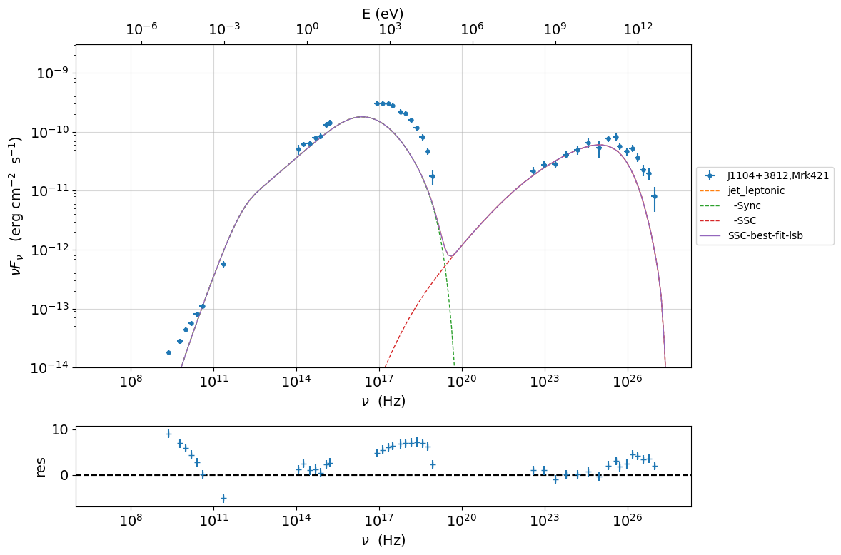
prefit_jet.eval()
pl=prefit_jet.plot_model(sed_data=sed_data)
pl.add_residual_plot(prefit_jet,sed_data)
pl.setlim(y_min=1E-15,x_min=1E7,x_max=1E29)

../../../../_images/Jet_example_model_fit_20_0.png

Model fitting procedure#

Note

Please, read the introduction and the caveat for the frequentist model fitting: to understand the frequentist fitting workflow see the Composite Models and depending pars user guide for further information about the implementation of FitModel, in particular for parameter setting

Model fitting with LSB#

from jetset.minimizer import fit_SED,ModelMinimizer

from jetset.model_manager import  FitModel
from jetset.jet_model import Jet

if you want to fit the prefit_model you can load the saved one (this allows you to save time) ad pass it to the FitModel class

prefit_jet=Jet.load_model('prefit_jet.pkl')
fit_model_lsb=FitModel( jet=prefit_jet, name='SSC-best-fit-lsb',template=None)

===> setting C threads to 12

OR use the one generated above

fit_model=FitModel( jet=prefit_jet, name='SSC-best-fit-lsb',template=None)

fit_model.show_model_components()

--------------------------------------------------------------------------------
Composite model description
--------------------------------------------------------------------------------
name: SSC-best-fit-lsb
type: composite_model
components models:
 -model name: jet_leptonic model type: jet

--------------------------------------------------------------------------------

There is only one component, whit name jet_leptonic, that refers to the prefit_jet model component

We now set the gamma grid size to 200, ad we set composite_expr, anyhow, since we have only one component this step could be skipped

fit_model.jet_leptonic.set_gamma_grid_size(200)
fit_model.composite_expr='jet_leptonic'

Freezeing parameters and setting fit_range intervals#

These methods are alternative and equivalent ways to access a model component for setting parameters state and values

passing as first argument, of the method, the model component name
passing as first argument, of the method, the model component object
accessing the model component member of the composite model class

#a
fit_model.freeze('jet_leptonic','z_cosm')
fit_model.freeze('jet_leptonic','R_H')
#b
fit_model.freeze(prefit_jet,'R')
#c
fit_model.jet_leptonic.parameters.R.fit_range=[10**15.5,10**17.5]
fit_model.jet_leptonic.parameters.beam_obj.fit_range=[5., 50.]

Building the ModelMinimizer object#

Now we build a lsb model minimizer and run the fit method

model_minimizer=ModelMinimizer('lsb')

Since the pre-fit model was very close to the data, we degrade the model in order to provide a more robust benchmark to the fitter, but this is not required!!!

fit_model.jet_leptonic.parameters.N.val=1
fit_model.jet_leptonic.parameters.r.val=1.0
fit_model.jet_leptonic.parameters.beam_obj.val=20
fit_model.eval()

%matplotlib inline
fit_model.set_nu_grid(1E6,1E30,200)
fit_model.eval()
p2=fit_model.plot_model(sed_data=sed_data)
p2.setlim(y_min=1E-14,x_min=1E6,x_max=2E28)

../../../../_images/Jet_example_model_fit_41_0.png

best_fit_res=model_minimizer.fit(fit_model,
                                     sed_data,
                                     1E11,
                                     1E29,
                                     fitname='SSC-best-fit-minuit',
                                     repeat=1)

filtering data in fit range = [1.000000e+11,1.000000e+29]
data length 35
================================================================================

* start fit process *
-----

0it [00:00, ?it/s]

- best chisq=2.72311e+01

-------------------------------------------------------------------------
Fit report

Model: SSC-best-fit-minuit

Table length=12

model name	name	par type	units	val	phys. bound. min	phys. bound. max	log	frozen
jet_leptonic	gmin	low-energy-cut-off	lorentz-factor*	6.477165e+02	1.000000e+00	1.000000e+09	False	False
jet_leptonic	gmax	high-energy-cut-off	lorentz-factor*	8.714388e+05	1.000000e+00	1.000000e+15	False	False
jet_leptonic	N	emitters_density	1 / cm3	5.375875e-01	0.000000e+00	--	False	False
jet_leptonic	gamma0_log_parab	turn-over-energy	lorentz-factor*	3.085231e+04	1.000000e+00	1.000000e+09	False	False
jet_leptonic	s	LE_spectral_slope		2.185631e+00	-1.000000e+01	1.000000e+01	False	False
jet_leptonic	r	spectral_curvature		5.620899e-01	-1.500000e+01	1.500000e+01	False	False
jet_leptonic	R	region_size	cm	3.460321e+16	1.000000e+03	1.000000e+30	False	True
jet_leptonic	R_H	region_position	cm	1.000000e+17	0.000000e+00	--	False	True
jet_leptonic	B	magnetic_field	gauss	5.027433e-02	0.000000e+00	--	False	False
jet_leptonic	NH_cold_to_rel_e	cold_p_to_rel_e_ratio		1.000000e+00	0.000000e+00	--	False	True
jet_leptonic	beam_obj	beaming		2.247307e+01	1.000000e-04	--	False	False
jet_leptonic	z_cosm	redshift		3.080000e-02	0.000000e+00	--	False	True

converged=True
calls=573
mesg=

'ftol termination condition is satisfied.'

dof=27
chisq=27.231050, chisq/red=1.008557 null hypothesis sig=0.451384

best fit pars

Table length=12

model name	name	val	bestfit val	err +	err -	start val	fit range min	fit range max	frozen
jet_leptonic	gmin	6.477165e+02	6.477165e+02	8.763882e+01	--	4.697542e+02	1.000000e+00	1.000000e+09	False
jet_leptonic	gmax	8.714388e+05	8.714388e+05	4.647860e+04	--	1.373160e+06	1.000000e+00	1.000000e+15	False
jet_leptonic	N	5.375875e-01	5.375875e-01	3.173721e-02	--	1.000000e+00	0.000000e+00	--	False
jet_leptonic	gamma0_log_parab	3.085231e+04	3.085231e+04	1.231389e+04	--	3.333017e+04	1.000000e+00	1.000000e+09	False
jet_leptonic	s	2.185631e+00	2.185631e+00	7.744080e-02	--	2.183468e+00	-1.000000e+01	1.000000e+01	False
jet_leptonic	r	5.620899e-01	5.620899e-01	9.878160e-02	--	1.000000e+00	-1.500000e+01	1.500000e+01	False
jet_leptonic	R	3.460321e+16	--	--	--	3.460321e+16	3.162278e+15	3.162278e+17	True
jet_leptonic	R_H	1.000000e+17	--	--	--	1.000000e+17	0.000000e+00	--	True
jet_leptonic	B	5.027433e-02	5.027433e-02	5.893700e-03	--	5.050000e-02	0.000000e+00	--	False
jet_leptonic	NH_cold_to_rel_e	1.000000e+00	--	--	--	1.000000e+00	0.000000e+00	--	True
jet_leptonic	beam_obj	2.247307e+01	2.247307e+01	1.523719e+00	--	2.000000e+01	5.000000e+00	5.000000e+01	False
jet_leptonic	z_cosm	3.080000e-02	--	--	--	3.080000e-02	0.000000e+00	--	True

-------------------------------------------------------------------------

================================================================================

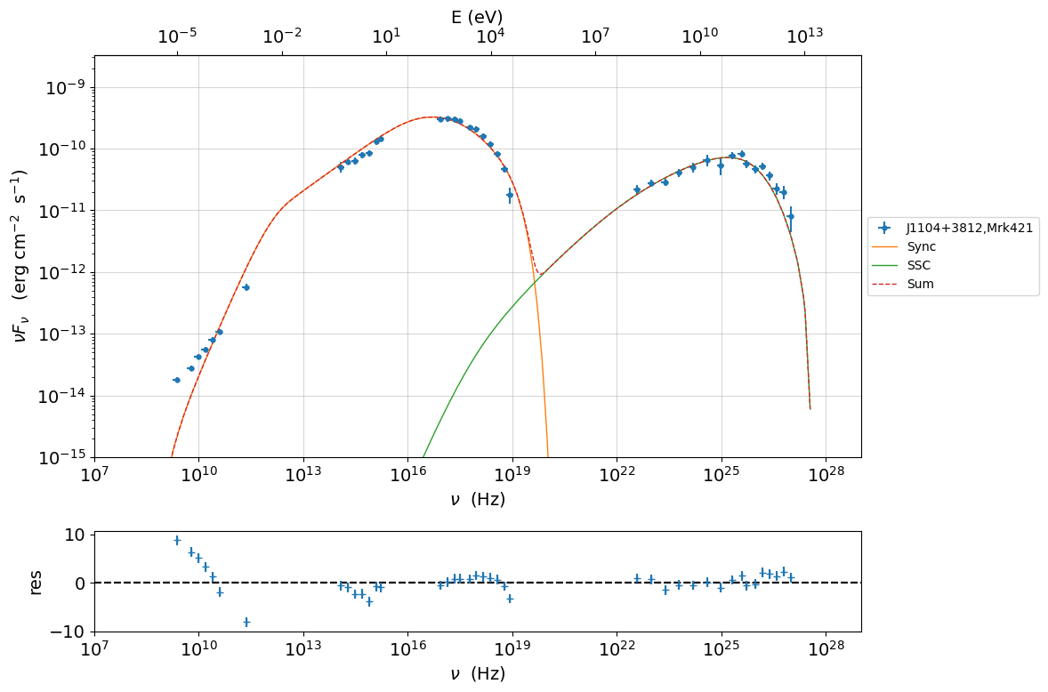
%matplotlib inline
fit_model.set_nu_grid(1E6,1E30,200)
fit_model.eval()
p2=fit_model.plot_model(sed_data=sed_data)
p2.setlim(y_min=1E-14,x_min=1E6,x_max=2E28)

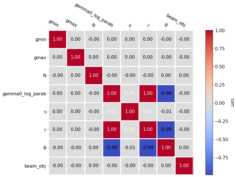
../../../../_images/Jet_example_model_fit_43_0.png

p=model_minimizer.plot_corr_matrix()

../../../../_images/Jet_example_model_fit_44_0.png

saving fit model, model minimizer#

We can save all the fit products to be used later.

best_fit_res.save_report('SSC-best-fit-lsb.pkl')
model_minimizer.save_model('model_minimizer_lsb.pkl')
fit_model.save_model('fit_model_lsb.pkl')

Model fitting with Minuit#

To run the minuit minimizer we will use the same prefit_jet model used for lsb

from jetset.minimizer import fit_SED,ModelMinimizer
from jetset.model_manager import  FitModel
from jetset.jet_model import Jet

jet_minuit=Jet.load_model('prefit_jet.pkl')
jet_minuit.set_gamma_grid_size(200)
fit_model_minuit=FitModel( jet=jet_minuit, name='SSC-best-fit-minuit',template=None)

===> setting C threads to 12

When using minuit, providing fit_range to parameters with large physical boundaries, such s ‘R’ or emitters Lorentz factors, is advised.

fit_model_minuit.freeze('jet_leptonic','z_cosm')
fit_model_minuit.freeze('jet_leptonic','R_H')
fit_model_minuit.freeze('jet_leptonic','R')
fit_model_minuit.jet_leptonic.parameters.R.fit_range=[5E15,1E17]
fit_model_minuit.jet_leptonic.parameters.gmin.fit_range=[10,1000]
fit_model_minuit.jet_leptonic.parameters.gmax.fit_range=[5E5,1E7]
fit_model_minuit.jet_leptonic.parameters.gamma0_log_parab.fit_range=[1E3,1E5]

fit_model_minuit.jet_leptonic.parameters.beam_obj.fit_range=[5,50]

Since the pre-fit model was very close to the data, we degrade the model in order to prove a more robust benchmark to the fitter

fit_model_minuit.jet_leptonic.parameters.N.val=1
fit_model_minuit.jet_leptonic.parameters.r.val=1.0
fit_model_minuit.jet_leptonic.parameters.beam_obj.val=20
fit_model_minuit.eval()

model_minimizer_minuit=ModelMinimizer('minuit')

best_fit_minuit=model_minimizer_minuit.fit(fit_model_minuit,
                                           sed_data,
                                           1E11,
                                           1E29,
                                           fitname='SSC-best-fit-minuit',
                                           max_ev=10000,
                                           repeat=2)

filtering data in fit range = [1.000000e+11,1.000000e+29]
data length 35
================================================================================

* start fit process *
-----
fit run: 0

0it [00:00, ?it/s]

====> simplex
====> migrad
- best chisq=2.88559e+01

fit run: 1
- old chisq=2.88559e+01

0it [00:00, ?it/s]

====> simplex
====> migrad
- best chisq=2.25297e+01

-------------------------------------------------------------------------
Fit report

Model: SSC-best-fit-minuit

Table length=12

model name	name	par type	units	val	phys. bound. min	phys. bound. max	log	frozen
jet_leptonic	gmin	low-energy-cut-off	lorentz-factor*	8.459850e+02	1.000000e+00	1.000000e+09	False	False
jet_leptonic	gmax	high-energy-cut-off	lorentz-factor*	9.786619e+05	1.000000e+00	1.000000e+15	False	False
jet_leptonic	N	emitters_density	1 / cm3	4.821025e-01	0.000000e+00	--	False	False
jet_leptonic	gamma0_log_parab	turn-over-energy	lorentz-factor*	7.202800e+04	1.000000e+00	1.000000e+09	False	False
jet_leptonic	s	LE_spectral_slope		2.329220e+00	-1.000000e+01	1.000000e+01	False	False
jet_leptonic	r	spectral_curvature		8.433724e-01	-1.500000e+01	1.500000e+01	False	False
jet_leptonic	R	region_size	cm	3.460321e+16	1.000000e+03	1.000000e+30	False	True
jet_leptonic	R_H	region_position	cm	1.000000e+17	0.000000e+00	--	False	True
jet_leptonic	B	magnetic_field	gauss	4.079311e-02	0.000000e+00	--	False	False
jet_leptonic	NH_cold_to_rel_e	cold_p_to_rel_e_ratio		1.000000e+00	0.000000e+00	--	False	True
jet_leptonic	beam_obj	beaming		2.531609e+01	1.000000e-04	--	False	False
jet_leptonic	z_cosm	redshift		3.080000e-02	0.000000e+00	--	False	True

converged=True
calls=687
mesg=

Migrad
FCN = 22.53		Nfcn = 687
EDM = 1.74 (Goal: 0.0002)		time = 15.1 sec
INVALID Minimum		No Parameters at limit
ABOVE EDM threshold (goal x 10)		Below call limit
Covariance	Hesse ok	Accurate	Pos. def.	Not forced

	Name	Value	Hesse Error	Minos Error-	Minos Error+	Limit-	Limit+	Fixed
0	par_0	845.984955	0.000010			10	1E+03
1	par_1	978.6619e3	0.0032e3			5E+05	1E+07
2	par_2	482.1025e-3	0.0010e-3			0
3	par_3	72e3	4e3			1E+03	1E+05
4	par_4	2.329220	0.000008			-10	10
5	par_5	843.3724e-3	0.0006e-3			-15	15
6	par_6	40.7931e-3	0.0024e-3			0
7	par_7	25.31609	0.00004			5	50

dof=27
chisq=22.529679, chisq/red=0.834433 null hypothesis sig=0.710002

best fit pars

Table length=12

model name	name	val	bestfit val	err +	err -	start val	fit range min	fit range max	frozen
jet_leptonic	gmin	8.459850e+02	8.459850e+02	1.043024e-05	--	4.697542e+02	1.000000e+01	1.000000e+03	False
jet_leptonic	gmax	9.786619e+05	9.786619e+05	3.166646e+00	--	1.373160e+06	5.000000e+05	1.000000e+07	False
jet_leptonic	N	4.821025e-01	4.821025e-01	1.049228e-06	--	1.000000e+00	0.000000e+00	--	False
jet_leptonic	gamma0_log_parab	7.202800e+04	7.202800e+04	4.302553e+03	--	3.333017e+04	1.000000e+03	1.000000e+05	False
jet_leptonic	s	2.329220e+00	2.329220e+00	7.853562e-06	--	2.183468e+00	-1.000000e+01	1.000000e+01	False
jet_leptonic	r	8.433724e-01	8.433724e-01	5.638138e-07	--	1.000000e+00	-1.500000e+01	1.500000e+01	False
jet_leptonic	R	3.460321e+16	--	--	--	3.460321e+16	5.000000e+15	1.000000e+17	True
jet_leptonic	R_H	1.000000e+17	--	--	--	1.000000e+17	0.000000e+00	--	True
jet_leptonic	B	4.079311e-02	4.079311e-02	2.411677e-06	--	5.050000e-02	0.000000e+00	--	False
jet_leptonic	NH_cold_to_rel_e	1.000000e+00	--	--	--	1.000000e+00	0.000000e+00	--	True
jet_leptonic	beam_obj	2.531609e+01	2.531609e+01	4.163996e-05	--	2.000000e+01	5.000000e+00	5.000000e+01	False
jet_leptonic	z_cosm	3.080000e-02	--	--	--	3.080000e-02	0.000000e+00	--	True

-------------------------------------------------------------------------

================================================================================

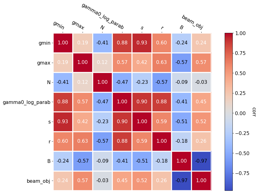
note that this plot refers to the latest fit trial, in case, please consider storing the plot within a list in the fit loop

p=model_minimizer_minuit.plot_corr_matrix()

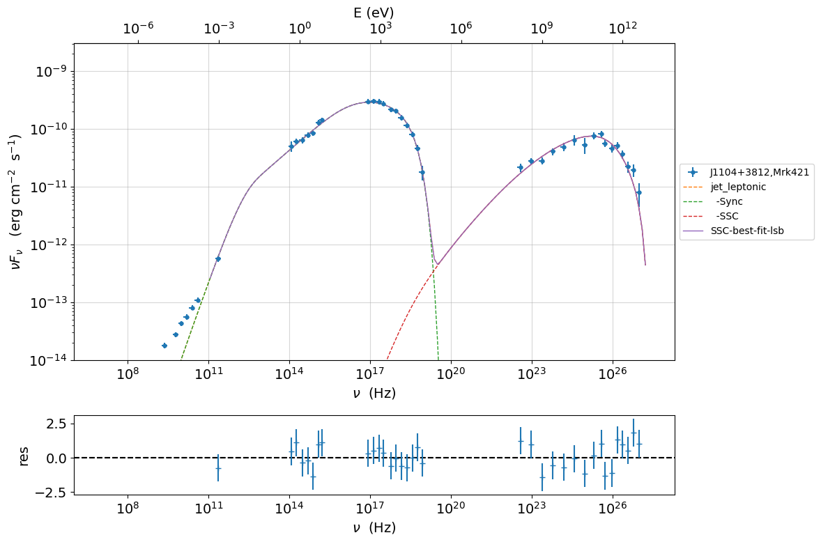
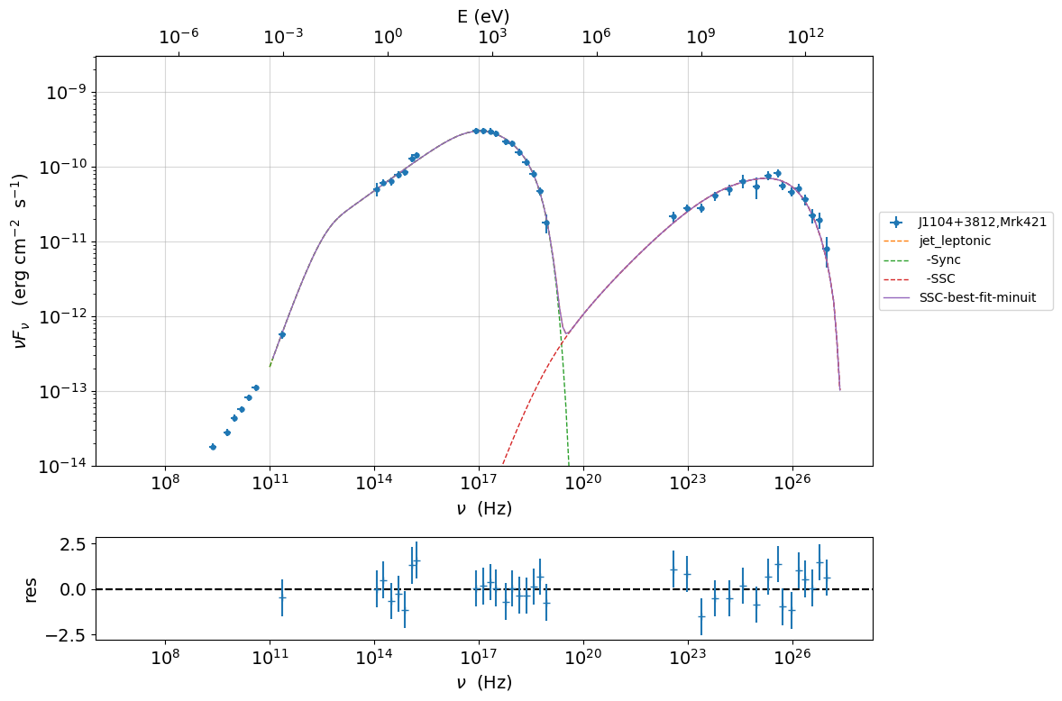
../../../../_images/Jet_example_model_fit_58_0.png

%matplotlib inline
fit_model_minuit.eval()
p2=fit_model_minuit.plot_model(sed_data=sed_data)
p2.setlim(y_min=1E-14,x_min=1E6,x_max=2E28)

../../../../_images/Jet_example_model_fit_59_0.png

saving fit model, model minimizer#

best_fit_minuit.save_report('SSC-best-fit-minuit.pkl')
model_minimizer_minuit.save_model('model_minimizer_minuit.pkl')
fit_model_minuit.save_model('fit_model_minuit.pkl')

You can obtain profile and contours, but this is typically time consuming. In any case, better results can be achieved using the MCMC approach (discussed in next section). For further information regarding minuit please refer to https://iminuit.readthedocs.io

#migrad profile

#access the data
profile_migrad=model_minimizer_minuit.minimizer.mnprofile('s')

#make the plot(no need to run the previous command)
profile_plot_migrad=model_minimizer_minuit.minimizer.draw_mnprofile('s')

#migrad contour
#access the data
contour_migrad=model_minimizer_minuit.minimizer.contour('beam_obj','B')

#make the plot(no need to run the previous command)
contour_plot_migrad=model_minimizer_minuit.minimizer.draw_contour('beam_obj','B')

you can use also minos contour and profile, in this case the computational time is even longer:

profile_migrad=model_minimizer_minuit.minimizer.mnprofile('s')
profile_plot_migrad=model_minimizer_minuit.minimizer.draw_mnprofile('s')

contour_migrad=model_minimizer_minuit.minimizer.mncontour('r','s')
contour_plot_migrad=model_minimizer_minuit.minimizer.draw_mncontour('r','s')

MCMC sampling#

Note

Please, read the introduction and the caveat for the Bayesian model fitting to understand the MCMC sampler workflow.

creating and setting the sampler#

from jetset.mcmc import McmcSampler
from jetset.minimizer import ModelMinimizer

model_minimizer_minuit = ModelMinimizer.load_model('model_minimizer_minuit.pkl')

mcmc=McmcSampler(model_minimizer_minuit)

===> setting C threads to 12

labels=['N','B','beam_obj','s','gamma0_log_parab']
model_name='jet_leptonic'
use_labels_dict={model_name:labels}

mcmc.set_labels(use_labels_dict=use_labels_dict)

mcmc.set_bounds(bound=5.0,bound_rel=True)

par: N  best fit value:  0.48210245803309054  mcmc bounds: [0, 2.892614748198543]
par: B  best fit value:  0.04079310894281457  mcmc bounds: [0, 0.24475865365688743]
par: beam_obj  best fit value:  25.316091554006853  mcmc bounds: [5, 50]
par: s  best fit value:  2.329220357129224  mcmc bounds: [-9.316881428516895, 10]
par: gamma0_log_parab  best fit value:  72028.00420425336  mcmc bounds: [1000.0, 100000.0]

mcmc.run_sampler(nwalkers=20, burnin=50,steps=500,progress='notebook')

===> setting C threads to 12
mcmc run starting

0%|          | 0/500 [00:00<?, ?it/s]

mcmc run done, with 1 threads took 216.05 seconds

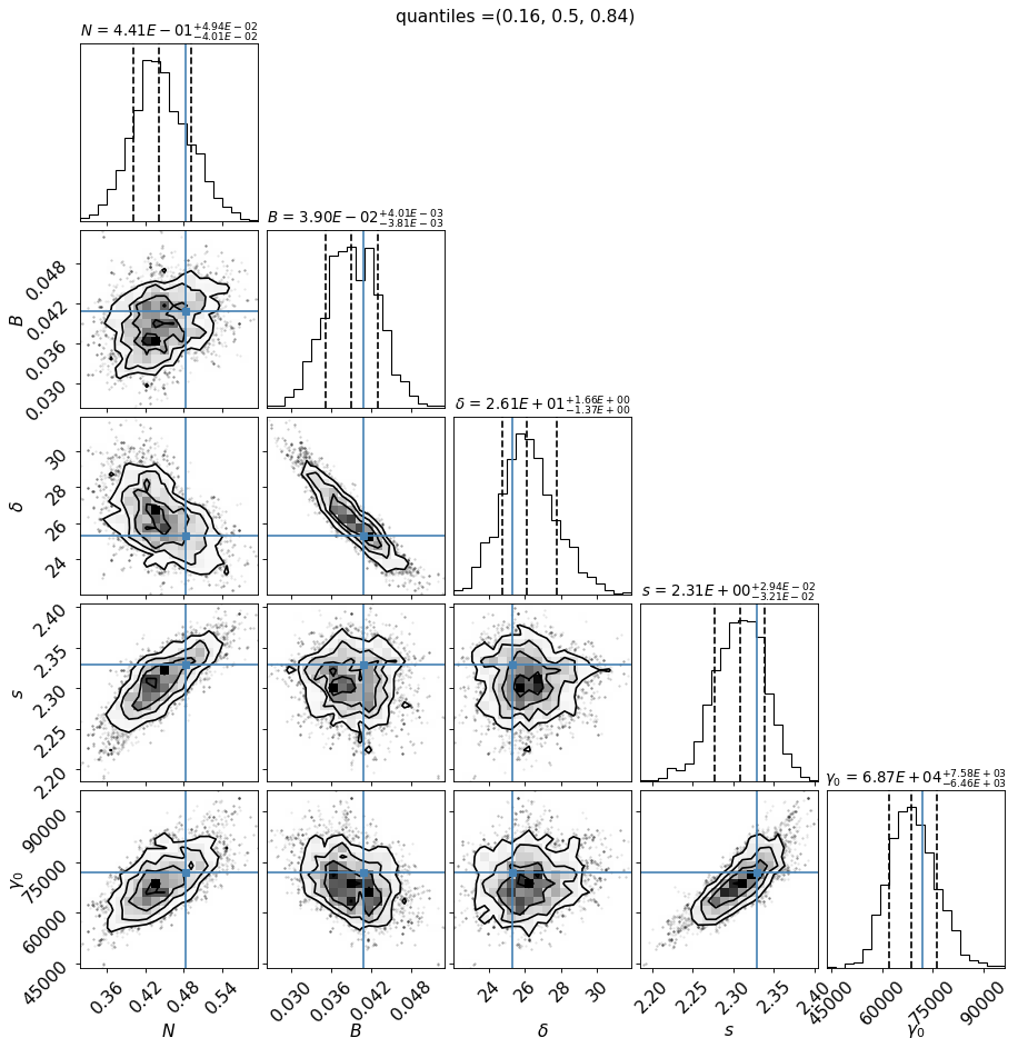
plotting the posterior corner plot#

printout the labels

mcmc.labels

['N', 'B', 'beam_obj', 's', 'gamma0_log_parab']

To have a better rendering on the scatter plot, we redefine the plot labels

mcmc.set_plot_label('N',r'$N$')
mcmc.set_plot_label('B',r'$B$')
mcmc.set_plot_label('beam_obj',r'$\delta$')
mcmc.set_plot_label('s',r'$s$')
mcmc.set_plot_label('gamma0_log_parab',r'$\gamma_0$')

the code below lets you tuning the output

mpl.rcParams[‘figure.dpi’] if you increase it you get a better definition
title_fmt=“.2E” this is the format for python, 2 significant digits, scientific notation
title_kwargs=dict(fontsize=12) you can change the fontsize

import matplotlib as mpl
mpl.rcParams['figure.dpi'] = 80
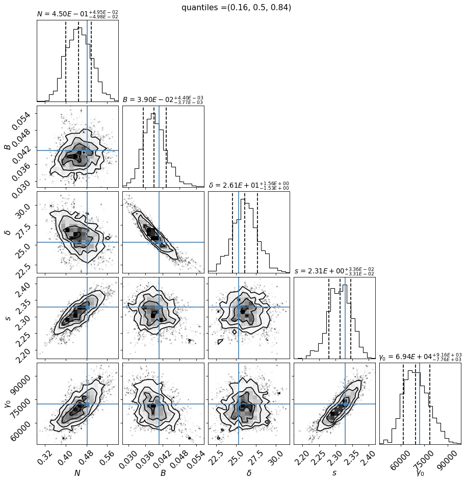
f=mcmc.corner_plot(quantiles=(0.16, 0.5, 0.84),title_kwargs=dict(fontsize=12),title_fmt=".2E",use_math_text=True)

../../../../_images/Jet_example_model_fit_81_0.png

print(mcmc.acceptance_fraction)

0.49329999999999996

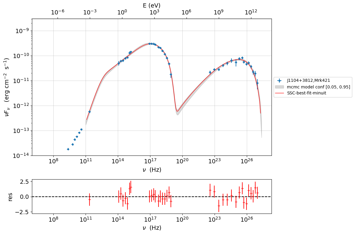
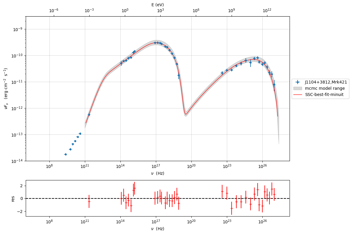
plotting the model#

To plot the sampled model against the input best-fit model

mpl.rcParams['figure.dpi'] = 80
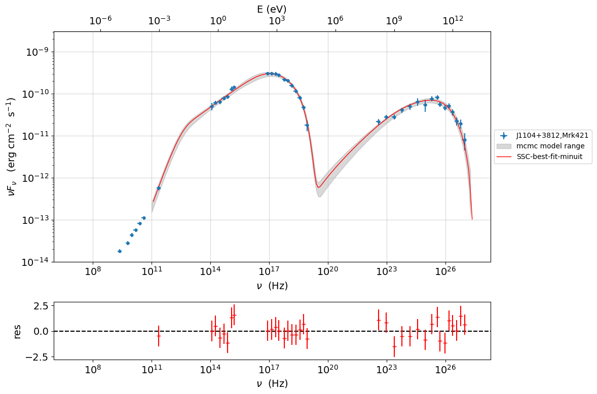
p=mcmc.plot_model(sed_data=sed_data,fit_range=[1E11,2E28],size=100)
p.setlim(y_min=1E-14,x_min=1E6,x_max=2E28)

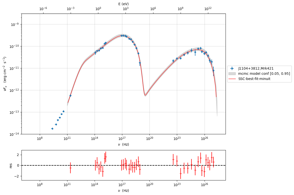
../../../../_images/Jet_example_model_fit_85_0.png

To plot the sampled model against the input best-fit model, providing quantiles

mpl.rcParams['figure.dpi'] = 80
p=mcmc.plot_model(sed_data=sed_data,fit_range=[1E11, 2E27],size=100,quantiles=[0.05,0.95])
p.setlim(y_min=1E-14,x_min=1E6,x_max=2E28)

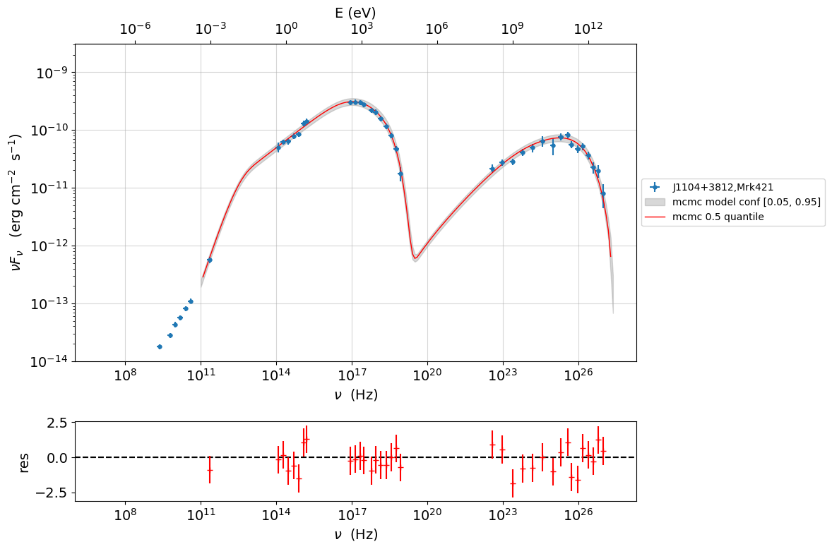
../../../../_images/Jet_example_model_fit_87_0.png

To plot the sampled model against the mcmc model at 0.5 quantile

mpl.rcParams['figure.dpi'] = 100
p=mcmc.plot_model(sed_data=sed_data,fit_range=[1E11, 2E27],size=100,quantiles=[0.05,0.95], plot_mcmc_best_fit_model=True)

p.setlim(y_min=1E-14,x_min=1E6,x_max=2E28)

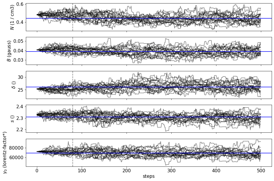
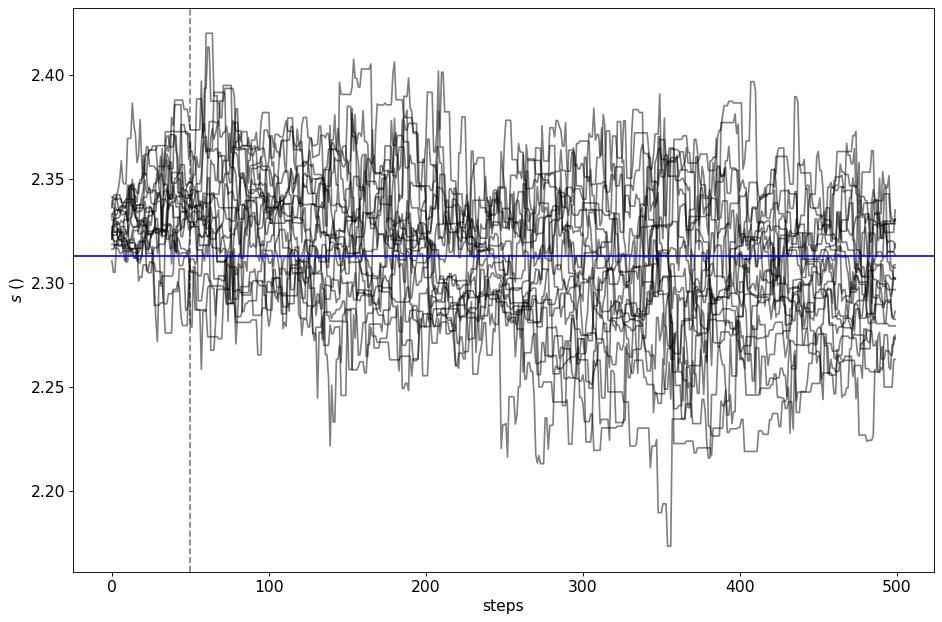
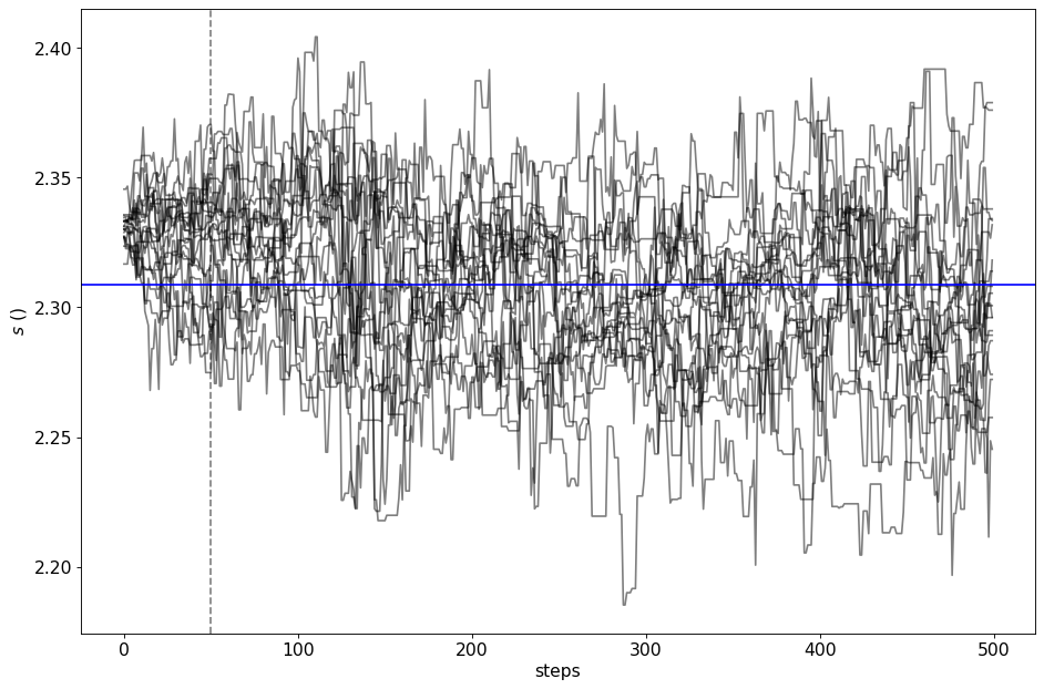
../../../../_images/Jet_example_model_fit_89_0.png

plotting chains and individual posteriors#

mpl.rcParams['figure.dpi'] = 80
f=mcmc.plot_chain(p='s',log_plot=False)
plt.tight_layout()

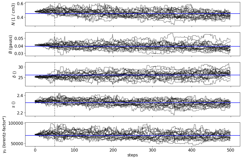
../../../../_images/Jet_example_model_fit_91_0.png

mpl.rcParams['figure.dpi'] = 80
f=mcmc.plot_chain(log_plot=False)
plt.tight_layout()

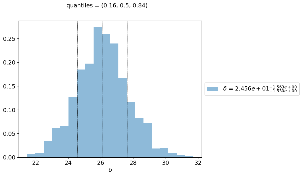
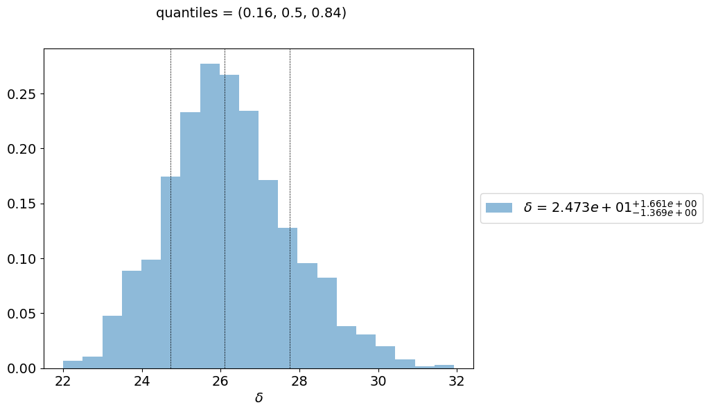
../../../../_images/Jet_example_model_fit_92_0.png

f=mcmc.plot_par('beam_obj',figsize=(8,6))
mpl.rcParams['figure.dpi'] = 80

../../../../_images/Jet_example_model_fit_93_0.png

mpl.rcParams['figure.dpi'] = 80
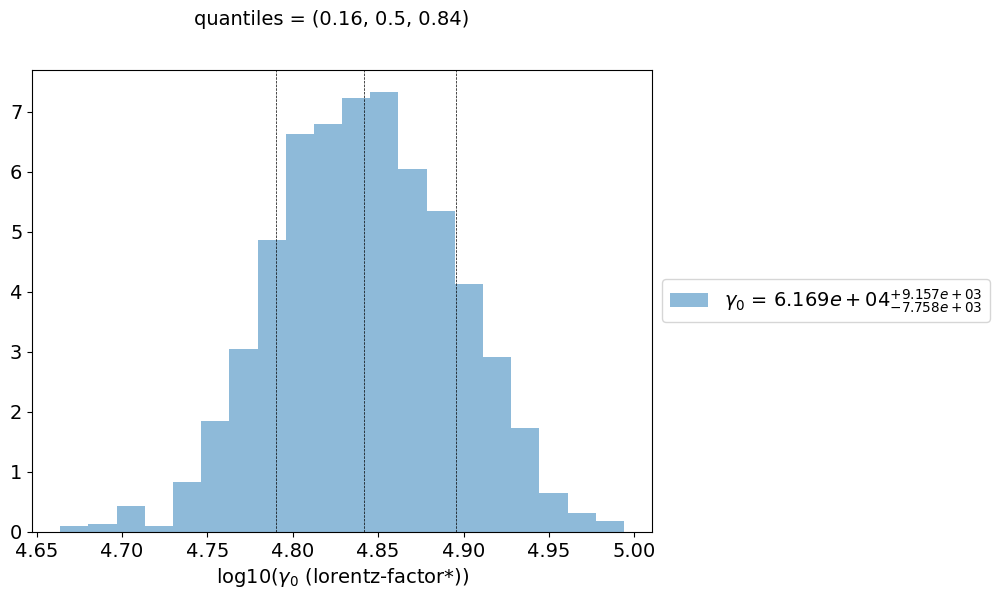
f=mcmc.plot_par('gamma0_log_parab',log_plot=True,figsize=(8,6))

../../../../_images/Jet_example_model_fit_94_0.png

Save and reuse MCMC#

mcmc.save('mcmc_sampler.pkl')

from jetset.mcmc import McmcSampler
from jetset.data_loader import ObsData
from jetset.plot_sedfit import PlotSED
from jetset.test_data_helper import  test_SEDs

sed_data=ObsData.load('Mrk_401.pkl')
ms=McmcSampler.load('mcmc_sampler.pkl')

import matplotlib as mpl

===> setting C threads to 12
===> setting C threads to 12

ms.model.name

'SSC-best-fit-minuit'

mpl.rcParams['figure.dpi'] = 80
p=ms.plot_model(sed_data=sed_data,fit_range=[1E11, 2E27],size=100)
p.setlim(y_min=1E-14,x_min=1E6,x_max=2E28)

../../../../_images/Jet_example_model_fit_99_0.png

mpl.rcParams['figure.dpi'] = 80
p=ms.plot_model(sed_data=sed_data,fit_range=[1E11, 2E27],size=100,quantiles=[0.05,0.95])

p.setlim(y_min=1E-14,x_min=1E6,x_max=2E28)

../../../../_images/Jet_example_model_fit_100_0.png

mpl.rcParams['figure.dpi'] = 80
p=ms.plot_model(sed_data=sed_data,fit_range=[1E11, 2E27],size=100,quantiles=[0.05,0.95],plot_mcmc_best_fit_model=True)

p.setlim(y_min=1E-14,x_min=1E6,x_max=2E28)

../../../../_images/Jet_example_model_fit_101_0.png

mpl.rcParams['figure.dpi'] = 80
f=ms.corner_plot(quantiles=(0.16, 0.5, 0.84),title_kwargs=dict(fontsize=12),title_fmt=".2E",use_math_text=True)

../../../../_images/Jet_example_model_fit_102_0.png

mpl.rcParams['figure.dpi'] = 80
f=ms.plot_par('beam_obj',log_plot=False,figsize=(8,6))

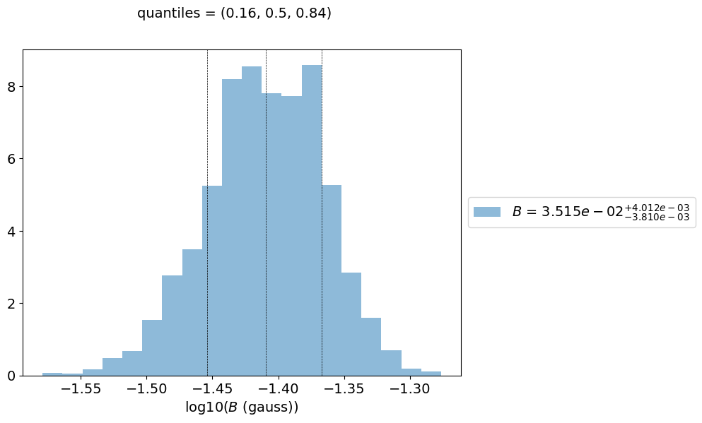
../../../../_images/Jet_example_model_fit_103_0.png

f=ms.plot_par('B',log_plot=True,figsize=(8,6))

../../../../_images/Jet_example_model_fit_104_0.png

mpl.rcParams['figure.dpi'] = 80
f=ms.plot_chain(p='s',log_plot=False)
plt.tight_layout()

../../../../_images/Jet_example_model_fit_105_0.png

f=ms.plot_chain(log_plot=False)
plt.tight_layout()
mpl.rcParams['figure.dpi'] = 80

../../../../_images/Jet_example_model_fit_106_0.png

Model fitting 1: Only SSC

Contents

Model fitting 1: Only SSC#

Loading data#

phenomenological model constraining#

spectral indices#

sed shaper#

Model constraining#

Model fitting procedure#

Model fitting with LSB#

Freezeing parameters and setting fit_range intervals#

Building the ModelMinimizer object#

saving fit model, model minimizer#

Model fitting with Minuit#

saving fit model, model minimizer#

MCMC sampling#

creating and setting the sampler#

plotting the posterior corner plot#

plotting the model#

plotting chains and individual posteriors#

Save and reuse MCMC#