Numerical setup#

import jetset
print('tested with',jetset.__version__)

tested with 1.4.0rc3

Changing the grid size for the electron distribution#

from jetset.jet_model import Jet
my_jet=Jet(name='test',electron_distribution='lppl',)
my_jet.show_model()

--------------------------------------------------------------------------------
model description:
--------------------------------------------------------------------------------
type: Jet
name: test
geometry: spherical

electrons distribution:
 type: lppl
 gamma energy grid size:  201
 gmin grid : 2.000000e+00
 gmax grid : 1.000000e+06
 normalization:  True
 log-values:  False
 ratio of cold protons to relativistic electrons: 1.000000e+00

radiative fields:
 seed photons grid size:  100
 IC emission grid size:  100
 source emissivity lower bound :  1.000000e-120
 spectral components:
   name:Sum, state: on
   name:Sum, hidden: False
   name:Sync, state: self-abs
   name:Sync, hidden: False
   name:SSC, state: on
   name:SSC, hidden: False
external fields transformation method: blob

SED info:
 nu grid size jetkernel: 1000
 nu size: 500
 nu mix (Hz): 1.000000e+06
 nu max (Hz): 1.000000e+30

flux plot lower bound   :  1.000000e-30

--------------------------------------------------------------------------------

WARNING: AstropyDeprecationWarning: 'classic' backend for show_in_notebook() is deprecated as of 6.1. Instead, use the supported backend 'ipydatagrid'. [astropy.table.table]

Table length=12

model name	name	par type	units	val	phys. bound. min	phys. bound. max	log	frozen
test	R	region_size	cm	5.000000e+15	1.000000e+03	1.000000e+30	False	False
test	R_H	region_position	cm	1.000000e+17	0.000000e+00	--	False	True
test	B	magnetic_field	gauss	1.000000e-01	0.000000e+00	--	False	False
test	NH_cold_to_rel_e	cold_p_to_rel_e_ratio		1.000000e+00	0.000000e+00	--	False	True
test	beam_obj	beaming		1.000000e+01	1.000000e-04	--	False	False
test	z_cosm	redshift		1.000000e-01	0.000000e+00	--	False	False
test	gmin	low-energy-cut-off	lorentz-factor*	2.000000e+00	1.000000e+00	1.000000e+09	False	False
test	gmax	high-energy-cut-off	lorentz-factor*	1.000000e+06	1.000000e+00	1.000000e+15	False	False
test	N	emitters_density	1 / cm3	1.000000e+02	0.000000e+00	--	False	False
test	gamma0_log_parab	turn-over-energy	lorentz-factor*	1.000000e+04	1.000000e+00	1.000000e+09	False	False
test	s	LE_spectral_slope		2.000000e+00	-1.000000e+01	1.000000e+01	False	False
test	r	spectral_curvature		4.000000e-01	-1.500000e+01	1.500000e+01	False	False

--------------------------------------------------------------------------------

It is possible to change the size of the grid for the electron distributions. It is worth noting that at lower values of the grid size the speed will increase, but it is not recommended to go below 100.

The actual value of the grid size is returned by the Jet.gamma_grid_size()

print (my_jet.gamma_grid_size)

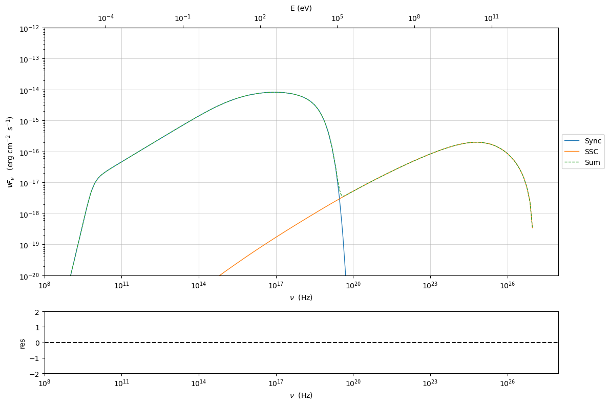
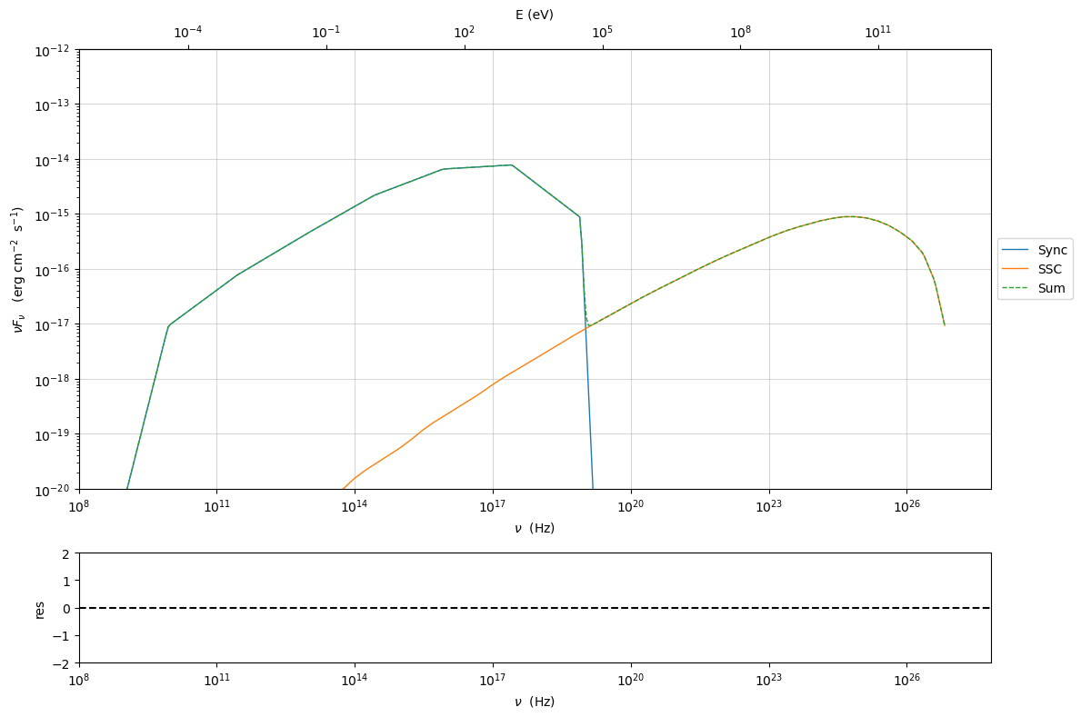
and this value can be changed using the method Jet.set_gamma_grid_size(). In the following we show the result for a grid of size=10, as anticipated the final integration will be not satisfactory

my_jet.set_gamma_grid_size(10)
my_jet.eval()
sed_plot=my_jet.plot_model()
sed_plot.setlim(x_min=1E8,y_min=1E-20,y_max=1E-12)

../../../../_images/Jet_example_num_9_0.png

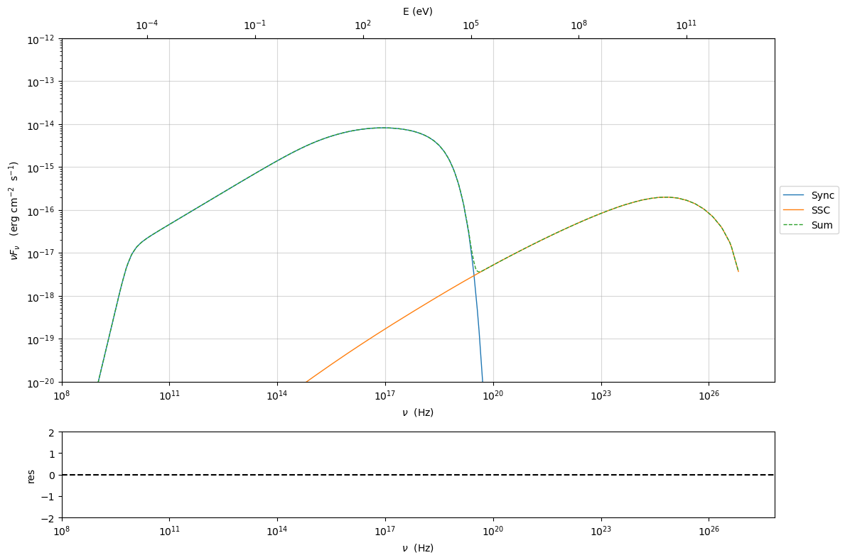
my_jet.set_gamma_grid_size(100)
my_jet.eval()
sed_plot=my_jet.plot_model()
sed_plot.setlim(x_min=1E8,y_min=1E-20,y_max=1E-12)

../../../../_images/Jet_example_num_10_0.png

Changing the grid size for the IC process spectra#

in the current version there is a limit of the size to 1000

my_jet=Jet(name='test',electron_distribution='lppl',)
my_jet.show_model()

--------------------------------------------------------------------------------
model description:
--------------------------------------------------------------------------------
type: Jet
name: test
geometry: spherical

electrons distribution:
 type: lppl
 gamma energy grid size:  201
 gmin grid : 2.000000e+00
 gmax grid : 1.000000e+06
 normalization:  True
 log-values:  False
 ratio of cold protons to relativistic electrons: 1.000000e+00

radiative fields:
 seed photons grid size:  100
 IC emission grid size:  100
 source emissivity lower bound :  1.000000e-120
 spectral components:
   name:Sum, state: on
   name:Sum, hidden: False
   name:Sync, state: self-abs
   name:Sync, hidden: False
   name:SSC, state: on
   name:SSC, hidden: False
external fields transformation method: blob

SED info:
 nu grid size jetkernel: 1000
 nu size: 500
 nu mix (Hz): 1.000000e+06
 nu max (Hz): 1.000000e+30

flux plot lower bound   :  1.000000e-30

--------------------------------------------------------------------------------

WARNING: AstropyDeprecationWarning: 'classic' backend for show_in_notebook() is deprecated as of 6.1. Instead, use the supported backend 'ipydatagrid'. [astropy.table.table]

Table length=12

model name	name	par type	units	val	phys. bound. min	phys. bound. max	log	frozen
test	R	region_size	cm	5.000000e+15	1.000000e+03	1.000000e+30	False	False
test	R_H	region_position	cm	1.000000e+17	0.000000e+00	--	False	True
test	B	magnetic_field	gauss	1.000000e-01	0.000000e+00	--	False	False
test	NH_cold_to_rel_e	cold_p_to_rel_e_ratio		1.000000e+00	0.000000e+00	--	False	True
test	beam_obj	beaming		1.000000e+01	1.000000e-04	--	False	False
test	z_cosm	redshift		1.000000e-01	0.000000e+00	--	False	False
test	gmin	low-energy-cut-off	lorentz-factor*	2.000000e+00	1.000000e+00	1.000000e+09	False	False
test	gmax	high-energy-cut-off	lorentz-factor*	1.000000e+06	1.000000e+00	1.000000e+15	False	False
test	N	emitters_density	1 / cm3	1.000000e+02	0.000000e+00	--	False	False
test	gamma0_log_parab	turn-over-energy	lorentz-factor*	1.000000e+04	1.000000e+00	1.000000e+09	False	False
test	s	LE_spectral_slope		2.000000e+00	-1.000000e+01	1.000000e+01	False	False
test	r	spectral_curvature		4.000000e-01	-1.500000e+01	1.500000e+01	False	False

--------------------------------------------------------------------------------

my_jet.eval()
sed_plot=my_jet.plot_model()
sed_plot.setlim(x_min=1E8,y_min=1E-20,y_max=1E-12)

../../../../_images/Jet_example_num_14_0.png

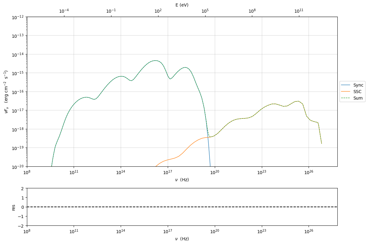
To get a better sampling of the IC cut-off you can increase the IC emission grid size

my_jet.set_IC_nu_size(200)

my_jet.eval()
sed_plot=my_jet.plot_model()
sed_plot.setlim(x_min=1E8,y_min=1E-20,y_max=1E-12)

../../../../_images/Jet_example_num_17_0.png

Changing the grid size for the seed photons#

my_jet=Jet(name='test',electron_distribution='lppl',)
my_jet.show_model()

--------------------------------------------------------------------------------
model description:
--------------------------------------------------------------------------------
type: Jet
name: test
geometry: spherical

electrons distribution:
 type: lppl
 gamma energy grid size:  201
 gmin grid : 2.000000e+00
 gmax grid : 1.000000e+06
 normalization:  True
 log-values:  False
 ratio of cold protons to relativistic electrons: 1.000000e+00

radiative fields:
 seed photons grid size:  100
 IC emission grid size:  100
 source emissivity lower bound :  1.000000e-120
 spectral components:
   name:Sum, state: on
   name:Sum, hidden: False
   name:Sync, state: self-abs
   name:Sync, hidden: False
   name:SSC, state: on
   name:SSC, hidden: False
external fields transformation method: blob

SED info:
 nu grid size jetkernel: 1000
 nu size: 500
 nu mix (Hz): 1.000000e+06
 nu max (Hz): 1.000000e+30

flux plot lower bound   :  1.000000e-30

--------------------------------------------------------------------------------

WARNING: AstropyDeprecationWarning: 'classic' backend for show_in_notebook() is deprecated as of 6.1. Instead, use the supported backend 'ipydatagrid'. [astropy.table.table]

Table length=12

model name	name	par type	units	val	phys. bound. min	phys. bound. max	log	frozen
test	R	region_size	cm	5.000000e+15	1.000000e+03	1.000000e+30	False	False
test	R_H	region_position	cm	1.000000e+17	0.000000e+00	--	False	True
test	B	magnetic_field	gauss	1.000000e-01	0.000000e+00	--	False	False
test	NH_cold_to_rel_e	cold_p_to_rel_e_ratio		1.000000e+00	0.000000e+00	--	False	True
test	beam_obj	beaming		1.000000e+01	1.000000e-04	--	False	False
test	z_cosm	redshift		1.000000e-01	0.000000e+00	--	False	False
test	gmin	low-energy-cut-off	lorentz-factor*	2.000000e+00	1.000000e+00	1.000000e+09	False	False
test	gmax	high-energy-cut-off	lorentz-factor*	1.000000e+06	1.000000e+00	1.000000e+15	False	False
test	N	emitters_density	1 / cm3	1.000000e+02	0.000000e+00	--	False	False
test	gamma0_log_parab	turn-over-energy	lorentz-factor*	1.000000e+04	1.000000e+00	1.000000e+09	False	False
test	s	LE_spectral_slope		2.000000e+00	-1.000000e+01	1.000000e+01	False	False
test	r	spectral_curvature		4.000000e-01	-1.500000e+01	1.500000e+01	False	False

--------------------------------------------------------------------------------

we can get the current value of the seed photons grid size using attribute Jet.nu_seed_size()

in the current version there is lit of the size to 1000

print (my_jet.nu_seed_size)

and this value can be changed using the method Jet.set_seed_nu_size(). In the following we show the result for a grid of nu_size=10

my_jet.nu_seed_size=10
my_jet.eval()
sed_plot=my_jet.plot_model()
sed_plot.setlim(x_min=1E8,y_min=1E-20,y_max=1E-12)

../../../../_images/Jet_example_num_24_0.png

my_jet=Jet(name='test',electron_distribution='lppl',)
my_jet.show_model()

--------------------------------------------------------------------------------
model description:
--------------------------------------------------------------------------------
type: Jet
name: test
geometry: spherical

electrons distribution:
 type: lppl
 gamma energy grid size:  201
 gmin grid : 2.000000e+00
 gmax grid : 1.000000e+06
 normalization:  True
 log-values:  False
 ratio of cold protons to relativistic electrons: 1.000000e+00

radiative fields:
 seed photons grid size:  100
 IC emission grid size:  100
 source emissivity lower bound :  1.000000e-120
 spectral components:
   name:Sum, state: on
   name:Sum, hidden: False
   name:Sync, state: self-abs
   name:Sync, hidden: False
   name:SSC, state: on
   name:SSC, hidden: False
external fields transformation method: blob

SED info:
 nu grid size jetkernel: 1000
 nu size: 500
 nu mix (Hz): 1.000000e+06
 nu max (Hz): 1.000000e+30

flux plot lower bound   :  1.000000e-30

--------------------------------------------------------------------------------

WARNING: AstropyDeprecationWarning: 'classic' backend for show_in_notebook() is deprecated as of 6.1. Instead, use the supported backend 'ipydatagrid'. [astropy.table.table]

Table length=12

model name	name	par type	units	val	phys. bound. min	phys. bound. max	log	frozen
test	R	region_size	cm	5.000000e+15	1.000000e+03	1.000000e+30	False	False
test	R_H	region_position	cm	1.000000e+17	0.000000e+00	--	False	True
test	B	magnetic_field	gauss	1.000000e-01	0.000000e+00	--	False	False
test	NH_cold_to_rel_e	cold_p_to_rel_e_ratio		1.000000e+00	0.000000e+00	--	False	True
test	beam_obj	beaming		1.000000e+01	1.000000e-04	--	False	False
test	z_cosm	redshift		1.000000e-01	0.000000e+00	--	False	False
test	gmin	low-energy-cut-off	lorentz-factor*	2.000000e+00	1.000000e+00	1.000000e+09	False	False
test	gmax	high-energy-cut-off	lorentz-factor*	1.000000e+06	1.000000e+00	1.000000e+15	False	False
test	N	emitters_density	1 / cm3	1.000000e+02	0.000000e+00	--	False	False
test	gamma0_log_parab	turn-over-energy	lorentz-factor*	1.000000e+04	1.000000e+00	1.000000e+09	False	False
test	s	LE_spectral_slope		2.000000e+00	-1.000000e+01	1.000000e+01	False	False
test	r	spectral_curvature		4.000000e-01	-1.500000e+01	1.500000e+01	False	False

--------------------------------------------------------------------------------

print(my_jet.IC_nu_size)

my_jet.IC_nu_size=20
my_jet.eval()
sed_plot=my_jet.plot_model()
sed_plot.setlim(x_min=1E8,y_min=1E-20,y_max=1E-12)

../../../../_images/Jet_example_num_27_0.png

my_jet.IC_nu_size=100
my_jet.eval()
sed_plot=my_jet.plot_model()
sed_plot.setlim(x_min=1E8,y_min=1E-20,y_max=1E-12)

../../../../_images/Jet_example_num_28_0.png

my_jet.IC_nu_size=200
my_jet.eval()
sed_plot=my_jet.plot_model()
sed_plot.setlim(x_min=1E8,y_min=1E-20,y_max=1E-12)

../../../../_images/Jet_example_num_29_0.png

my_jet._blob.core.IC_adaptive_e_binning
my_jet.IC_nu_size=100
my_jet.eval()
sed_plot=my_jet.plot_model()
sed_plot.setlim(x_min=1E8,y_min=1E-20,y_max=1E-12)

../../../../_images/Jet_example_num_30_0.png

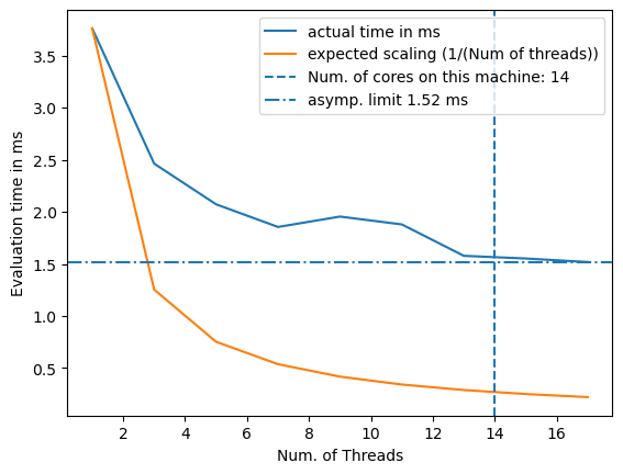
Tuning the C threads number#

The code below shows how to profile the computational time in terms of the number of C threads. The default value used by jetset, that is setting the number of C thread equal to the number of cores in the machine, is already providing the best performance.

import matplotlib.pylab as plt
import time
import numpy as np
import multiprocessing
th_arr=[1,2,4,8,14,16,32]
t_ev=[]

#number of cores on the machine
#this might change on clusters or docker, please be aware of!
N_cores=multiprocessing.cpu_count()

th_arr=np.arange(1,N_cores+4,2,dtype=np.int32)
my_jet=Jet()
for th in th_arr:
    t_spent=0
    N=500
    my_jet.set_num_c_threads(int(th),verbose=False)

    t_start=time.perf_counter()
    for i in range(N):
        my_jet.eval()
    t_spent=(time.perf_counter() -t_start)
    t_ms=t_spent/N*1000
    t_ev.append(t_ms)
plt.plot(th_arr,t_ev,label='actual time in ms')
plt.plot(th_arr,t_ev[0]/np.array(th_arr),label='expected scaling (1/(Num of threads))')
plt.xlabel('Num. of Threads')
plt.ylabel('Evaluation time in ms')
plt.axvline(N_cores,ls='--',label=f'Num. of cores on this machine: {N_cores}')
plt.axhline(t_ev[-1], ls='-.', label=f'asymp. limit {t_ev[-1]:.2f} ms')
plt.legend()

<matplotlib.legend.Legend at 0x163c8d070>

../../../../_images/Jet_example_num_33_1.png

Numerical setup

Contents

Numerical setup#

Changing the grid size for the electron distribution#

Changing the grid size for the IC process spectra#

Changing the grid size for the seed photons#

Tuning the C threads number#